数据结构简介
我们将首先快速,非全面地概述大熊猫中的基本数据结构,以帮助您入门。关于数据类型,索引和轴标记/对齐的基本行为适用于所有对象。首先,导入NumPy并将pandas加载到命名空间中:
import numpy as np
import pandas as pd这是一个要记住的基本原则:数据对齐是固有的。除非您明确说明,否则标签和数据之间的链接不会被破坏。
我们将简要介绍数据结构,然后在单独的部分中考虑所有大类功能和方法。
两种主要的数据结构:
- Series
- DataFrame
Series
Series是一维标记的数组,能够保存任何数据类型(整数,字符串,浮点数,Python对象等)。轴标签统称为索引。创建系列的基本方法是调用:
s = pd.Series(data, index=index)在这里,data可以有很多不同的东西:
- Python字典
- ndarray
- 标量值(如5)
传递的索引是轴标签列表。因此,根据数据的不同,这可分为几种情况:
来自ndarray(数组)
如果data是ndarray,则索引的长度必须与数据的长度相同。如果没有传递索引,将创建一个具有值的索引。[0, ...,len(data) - 1]
In [3]: s = pd.Series(np.random.randn(5), index=['a', 'b', 'c', 'd', 'e'])

In [4]: s
Out[4]:
a    0.4691
b   -0.2829
c   -1.5091
d   -1.1356
e    1.2121
dtype: float64

In [5]: s.index
Out[5]: Index(['a', 'b', 'c', 'd', 'e'], dtype='object')

In [6]: pd.Series(np.random.randn(5))
Out[6]:
0   -0.1732
1    0.1192
2   -1.0442
3   -0.8618
4   -2.1046
dtype: float64注意:pandas支持非唯一索引值。如果尝试不支持重复索引值的操作,则会在此时引发异常。懒惰的原因几乎都是基于性能的(计算中有很多实例,比如GroupBy中没有使用索引的部分)。
来自Dict(字典)
Series可以从dicts实例化:
In [7]: d = {'b' : 1, 'a' : 0, 'c' : 2}

In [8]: pd.Series(d)
Out[8]:
b    1
a    0
c    2
dtype: int64注意:当数据是dict,并且未传递Series索引时,如果您使用的是Python版本> = 3.6且Pandas版本> = 0.23 ,则索引将按dict的插入顺序排序。
如果您使用的是Python <3.6或Pandas <0.23,并且未传递Series索引,则索引将是词汇顺序的dict键列表。
在上面的示例中,如果您使用的Python版本低于3.6或Pandas版本低于0.23,Series则将按字典键的词法顺序(即而不是)进行排序。['a', 'b', 'c']['b', 'a', 'c']
如果传递索引,则将拉出与索引中的标签对应的数据中的值。
In [9]: d = {'a' : 0., 'b' : 1., 'c' : 2.}

In [10]: pd.Series(d)
Out[10]:
a    0.0
b    1.0
c    2.0
dtype: float64

In [11]: pd.Series(d, index=['b', 'c', 'd', 'a'])
Out[11]:
b    1.0
c    2.0
d    NaN
a    0.0
dtype: float64注意:NaN(不是数字)是pandas中使用的标准缺失数据标记。
来自标量值
如果data是标量值,则必须提供索引。将重复该值以匹配索引的长度。
In [12]: pd.Series(5., index=['a', 'b', 'c', 'd', 'e'])
Out[12]:
a    5.0
b    5.0
c    5.0
d    5.0
e    5.0
dtype: float64
Series类似ndarray
Series行为与a非常相似ndarray,并且是大多数NumPy函数的有效参数。但是,切片等操作也会对索引进行切片。
In [13]: s[0]
Out[13]: 0.46911229990718628

In [14]: s[:3]
Out[14]:
a    0.4691
b   -0.2829
c   -1.5091
dtype: float64

In [15]: s[s > s.median()]
Out[15]:
a    0.4691
e    1.2121
dtype: float64

In [16]: s[[4, 3, 1]]
Out[16]:
e    1.2121
d   -1.1356
b   -0.2829
dtype: float64

In [17]: np.exp(s)
Out[17]:
a    1.5986
b    0.7536
c    0.2211
d    0.3212
e    3.3606
dtype: float64我们将在单独的部分中讨论基于数组的索引。
Series 类似 Dict
Series类似于固定大小的dict,您可以通过索引标签获取和设置值:
In [18]: s['a']
Out[18]: 0.46911229990718628

In [19]: s['e'] = 12.

In [20]: s
Out[20]:
a     0.4691
b    -0.2829
c    -1.5091
d    -1.1356
e    12.0000
dtype: float64

In [21]: 'e' in s
Out[21]: True

In [22]: 'f' in s
Out[22]: False
如果未包含标签,则会引发异常:
>>> s['f']
KeyError: 'f'使用该get方法,缺少的标签将返回None或指定的默认值:
In [23]: s.get('f')

In [24]: s.get('f', np.nan)
Out[24]: nan使用Series进行矢量化操作和标签对齐
使用原始NumPy数组时,通常不需要循环使用value-by-value。在pandas中使用Series时也是如此。Series 也可以传递到大多数期待ndarray的NumPy方法。
In [25]: s + s
Out[25]:
a     0.9382
b    -0.5657
c    -3.0181
d    -2.2713
e    24.0000
dtype: float64

In [26]: s * 2
Out[26]:
a     0.9382
b    -0.5657
c    -3.0181
d    -2.2713
e    24.0000
dtype: float64

In [27]: np.exp(s)
Out[27]:
a         1.5986
b         0.7536
c         0.2211
d         0.3212
e    162754.7914
dtype: float64Series和ndarray之间的主要区别在于Series之间的操作会根据标签自动对齐数据。因此,您可以在不考虑所涉及的Series 是否具有相同标签的情况下编写计算。
In [28]: s[1:] + s[:-1]
Out[28]:
a       NaN
b   -0.5657
c   -3.0181
d   -2.2713
e       NaN
dtype: float64
未对齐Series 之间的操作结果将包含所涉及的索引的并集。如果在一个Series 或另一个Series 中找不到标签,则结果将标记为缺失NaN。能够在不进行任何明确数据对齐的情况下编写代码,可以在交互式数据分析和研究中获得巨大的自由度和灵活性。除了用于处理标记数据的大多数相关工具之外,大熊猫数据结构的集成数据对齐功能设置了熊猫。
注意:通常,我们选择使不同索引对象之间的操作的默认结果产生索引的并集,以避免信息丢失。尽管缺少数据,但索引标签通常是重要信息,作为计算的一部分。您当然可以选择通过dropna函数删除缺少数据的标签 。
名称属性
Series也可以有一个name属性:
In [29]: s = pd.Series(np.random.randn(5), name='something')

In [30]: s
Out[30]:
0   -0.4949
1    1.0718
2    0.7216
3   -0.7068
4   -1.0396
Name: something, dtype: float64

In [31]: s.name
Out[31]: 'something'name在许多情况下,Series 将自动分配,特别是在拍摄一维DataFrame时,如下所示。
版本0.18.0中的新功能。
您可以使用该pandas.Series.rename()方法重命名Series 。
In [32]: s2 = s.rename("different")

In [33]: s2.name
Out[33]: 'different'请注意s并s2引用不同的对象。
DataFrame
DataFrame是一个二维标记数据结构,具有可能不同类型的列。您可以将其视为电子表格或SQL表,或Series对象的字典。它通常是最常用的pandas对象。与Series类似,DataFrame接受许多不同类型的输入:
- 1D ndarray,list,dicts或Series的Dict
- 二维numpy.ndarray
- 结构化或记录 ndarray
- 一个
Series - 另一个
DataFrame
除了数据,您还可以选择传递索引(行标签)和 列(列标签)参数。如果传递索引和/或列,则可以保证生成的DataFrame的索引和/或列。因此,系列的字典加上特定索引将丢弃与传递的索引不匹配的所有数据。
如果未传递轴标签,则将根据常识规则从输入数据构造它们。
注意:当数据是dict columns且未指定时,DataFrame 如果您使用的是Python版本> = 3.6且Pandas> = 0.23 ,则列将按dict的插入顺序排序。
如果您使用的是Python <3.6或Pandas <0.23,并且columns未指定,则DataFrame列将是词汇顺序的dict键列表。
来自 Series 或 dict 的字典
得到的index将是联合的各种Series的指标。如果有任何嵌套的dicts,这些将首先转换为Series。如果没有传递列,则列将是dict键的有序列表。
In [34]: d = {'one' : pd.Series([1., 2., 3.], index=['a', 'b', 'c']),
   ....:      'two' : pd.Series([1., 2., 3., 4.], index=['a', 'b', 'c', 'd'])}
   ....:

In [35]: df = pd.DataFrame(d)

In [36]: df
Out[36]:
   one  two
a  1.0  1.0
b  2.0  2.0
c  3.0  3.0
d  NaN  4.0

In [37]: pd.DataFrame(d, index=['d', 'b', 'a'])
Out[37]:
   one  two
d  NaN  4.0
b  2.0  2.0
a  1.0  1.0

In [38]: pd.DataFrame(d, index=['d', 'b', 'a'], columns=['two', 'three'])
Out[38]:
   two three
d  4.0   NaN
b  2.0   NaN
a 1.0 NaN通过访问索引和列属性,可以分别访问行和列标签 :
注意:当一组特定的列与数据的dict一起传递时,传递的列将覆盖dict中的键。
In [39]: df.index
Out[39]: Index(['a', 'b', 'c', 'd'], dtype='object')

In [40]: df.columns
Out[40]: Index(['one', 'two'], dtype='object')
来自 ndarrays/lists 的字典
ndarrays必须都是相同的长度。如果传递索引,则它必须明显与数组的长度相同。如果没有传递索引,结果将是range(n),n数组长度在哪里。
In [41]: d = {'one' : [1., 2., 3., 4.],
   ....:      'two' : [4., 3., 2., 1.]}
   ....:

In [42]: pd.DataFrame(d)
Out[42]:
   one  two
0  1.0  4.0
1  2.0  3.0
2  3.0  2.0
3  4.0  1.0

In [43]: pd.DataFrame(d, index=['a', 'b', 'c', 'd'])
Out[43]:
   one  two
a  1.0  4.0
b  2.0  3.0
c  3.0  2.0
d  4.0  1.0
来自结构化或记录数组
这种情况的处理方式与数组的字典相同。
In [44]: data = np.zeros((2,), dtype=[('A', 'i4'),('B', 'f4'),('C', 'a10')])

In [45]: data[:] = [(1,2.,'Hello'), (2,3.,"World")]

In [46]: pd.DataFrame(data)
Out[46]:
   A    B         C
0  1  2.0  b'Hello'
1  2  3.0  b'World'

In [47]: pd.DataFrame(data, index=['first', 'second'])
Out[47]:
        A    B         C
first   1  2.0  b'Hello'
second  2  3.0  b'World'

In [48]: pd.DataFrame(data, columns=['C', 'A', 'B'])
Out[48]:
          C  A    B
0  b'Hello'  1  2.0
1 b'World' 2 3.0注意:DataFrame并不像二维NumPy ndarray那样工作。
来自dicts列表
In [49]: data2 = [{'a': 1, 'b': 2}, {'a': 5, 'b': 10, 'c': 20}]

In [50]: pd.DataFrame(data2)
Out[50]:
   a   b     c
0  1   2   NaN
1  5  10  20.0

In [51]: pd.DataFrame(data2, index=['first', 'second'])
Out[51]:
        a   b     c
first   1   2   NaN
second  5  10  20.0

In [52]: pd.DataFrame(data2, columns=['a', 'b'])
Out[52]:
   a   b
0  1   2
1  5  10
来自元组的词典
您可以通过传递元组字典自动创建多索引框架。
In [53]: pd.DataFrame({('a', 'b'): {('A', 'B'): 1, ('A', 'C'): 2},
   ....:               ('a', 'a'): {('A', 'C'): 3, ('A', 'B'): 4},
   ....:               ('a', 'c'): {('A', 'B'): 5, ('A', 'C'): 6},
   ....:               ('b', 'a'): {('A', 'C'): 7, ('A', 'B'): 8},
   ....:               ('b', 'b'): {('A', 'D'): 9, ('A', 'B'): 10}})
   ....:
Out[53]:
       a              b
       b    a    c    a     b
A B  1.0  4.0  5.0  8.0  10.0
  C  2.0  3.0  6.0  7.0   NaN
  D  NaN  NaN  NaN  NaN   9.0
来自Series
结果将是一个与输入Series具有相同索引的DataFrame,以及一个列,其名称是Series的原始名称(仅当没有提供其他列名时)。
缺失数据
在“ 缺失数据” 部分中将对此主题进行更多说明。要构造包含缺失数据的DataFrame,我们使用它np.nan来表示缺失值。或者,您可以将a numpy.MaskedArray 作为data参数传递给DataFrame构造函数,并且其被屏蔽的条目将被视为缺失。
备用构造函数
DataFrame.from_dict
DataFrame.from_dict采用dicts的dict或类似数组序列的dict并返回DataFrame。DataFrame除了默认情况下的orient参数外,它的操作类似于构造函数'columns',但可以将其设置'index'为使用dict键作为行标签。
In [54]: pd.DataFrame.from_dict(dict([('A', [1, 2, 3]), ('B', [4, 5, 6])]))
Out[54]:
   A  B
0  1  4
1  2  5
2 3 6如果通过orient='index',则键将是行标签。在这种情况下,您还可以传递所需的列名称:
In [55]: pd.DataFrame.from_dict(dict([('A', [1, 2, 3]), ('B', [4, 5, 6])]),
   ....:                        orient='index', columns=['one', 'two', 'three'])
   ....:
Out[55]:
   one  two  three
A    1    2      3
B    4    5      6
DataFrame.from_records
DataFrame.from_records获取元组列表或带有结构化dtype的ndarray。它类似于普通DataFrame构造函数,但生成的DataFrame索引可能是结构化dtype的特定字段。例如:
In [56]: data
Out[56]:
array([(1,  2., b'Hello'), (2,  3., b'World')],
      dtype=[('A', '<i4'), ('B', '<f4'), ('C', 'S10')])

In [57]: pd.DataFrame.from_records(data, index='C')
Out[57]:
          A    B
C
b'Hello'  1  2.0
b'World'  2  3.0
列选择,添加,删除
您可以在语义上将DataFrame视为类似索引的Series对象的dict。获取,设置和删除列的工作方式与类似的dict操作相同:
In [58]: df['one']
Out[58]:
a    1.0
b    2.0
c    3.0
d    NaN
Name: one, dtype: float64

In [59]: df['three'] = df['one'] * df['two']

In [60]: df['flag'] = df['one'] > 2

In [61]: df
Out[61]:
   one  two  three   flag
a  1.0  1.0    1.0  False
b  2.0  2.0    4.0  False
c  3.0  3.0    9.0   True
d  NaN  4.0    NaN  False
列可以像dict一样删除或弹出:
In [62]: del df['two']

In [63]: three = df.pop('three')

In [64]: df
Out[64]:
   one   flag
a  1.0  False
b  2.0  False
c  3.0   True
d  NaN  False
插入标量值时,它会自然地传播以填充列:
In [65]: df['foo'] = 'bar'

In [66]: df
Out[66]:
   one   flag  foo
a  1.0  False  bar
b  2.0  False  bar
c  3.0   True  bar
d  NaN  False  bar
插入与DataFrame不具有相同索引的Series时,它将符合DataFrame的索引:
In [67]: df['one_trunc'] = df['one'][:2]

In [68]: df
Out[68]:
   one   flag  foo  one_trunc
a  1.0  False  bar        1.0
b  2.0  False  bar        2.0
c  3.0   True  bar        NaN
d  NaN  False  bar        NaN
您可以插入原始ndarrays,但它们的长度必须与DataFrame索引的长度相匹配。
默认情况下,列会在末尾插入。该insert函数可用于插入列中的特定位置:
In [69]: df.insert(1, 'bar', df['one'])

In [70]: df
Out[70]:
   one  bar   flag  foo  one_trunc
a  1.0  1.0  False  bar        1.0
b  2.0  2.0  False  bar        2.0
c  3.0  3.0   True  bar        NaN
d  NaN  NaN  False  bar        NaN
在方法链中分配新列
受dplyr mutate动词的启发,DataFrame有一种assign() 方法可以让您轻松创建可能从现有列派生的新列。
In [71]: iris = pd.read_csv('data/iris.data')

In [72]: iris.head()
Out[72]:
   SepalLength  SepalWidth  PetalLength  PetalWidth         Name
0          5.1         3.5          1.4         0.2  Iris-setosa
1          4.9         3.0          1.4         0.2  Iris-setosa
2          4.7         3.2          1.3         0.2  Iris-setosa
3          4.6         3.1          1.5         0.2  Iris-setosa
4          5.0         3.6          1.4         0.2  Iris-setosa

In [73]: (iris.assign(sepal_ratio = iris['SepalWidth'] / iris['SepalLength'])
   ....:      .head())
   ....:
Out[73]:
   SepalLength  SepalWidth  PetalLength  PetalWidth         Name  sepal_ratio
0          5.1         3.5          1.4         0.2  Iris-setosa       0.6863
1          4.9         3.0          1.4         0.2  Iris-setosa       0.6122
2          4.7         3.2          1.3         0.2  Iris-setosa       0.6809
3          4.6         3.1          1.5         0.2  Iris-setosa       0.6739
4          5.0         3.6          1.4         0.2  Iris-setosa       0.7200
在上面的示例中,我们插入了一个预先计算的值。我们还可以传入一个参数的函数,以便在分配给的DataFrame上进行求值。
In [74]: iris.assign(sepal_ratio = lambda x: (x['SepalWidth'] /
   ....:                                      x['SepalLength'])).head()
   ....:
Out[74]:
   SepalLength  SepalWidth  PetalLength  PetalWidth         Name  sepal_ratio
0          5.1         3.5          1.4         0.2  Iris-setosa       0.6863
1          4.9         3.0          1.4         0.2  Iris-setosa       0.6122
2          4.7         3.2          1.3         0.2  Iris-setosa       0.6809
3          4.6         3.1          1.5         0.2  Iris-setosa       0.6739
4          5.0         3.6          1.4         0.2  Iris-setosa       0.7200
assign 始终返回数据的副本,保持原始DataFrame不变。
当您没有对手头的DataFrame的引用时,传递可调用的,而不是要插入的实际值。这assign在操作链中使用时很常见。例如,我们可以将DataFrame限制为仅包含Sepal Length大于5的观察值,计算比率,并绘制:
In [75]: (iris.query('SepalLength > 5')
   ....:      .assign(SepalRatio = lambda x: x.SepalWidth / x.SepalLength,
   ....:              PetalRatio = lambda x: x.PetalWidth / x.PetalLength)
   ....:      .plot(kind='scatter', x='SepalRatio', y='PetalRatio'))
   ....:
Out[75]: <matplotlib.axes._subplots.AxesSubplot at 0x7f210fb001d0>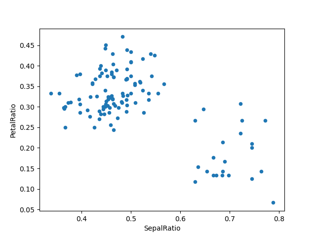
由于传入函数,因此在分配给的DataFrame上计算函数。重要的是,这是已经过滤到那些萼片长度大于5的行的DataFrame。首先进行过滤,然后进行比率计算。这是一个我们没有对可用的过滤 DataFrame 的引用的示例。
功能签名assign很简单**kwargs。键是新字段的列名,值是要插入的值(例如,a Series或NumPy数组),或者是要在其上调用的一个参数的函数DataFrame。一个副本的原始数据帧的返回,插入新的值。
版本0.23.0已更改。
从Python 3.6开始,**kwargs保留了顺序。这允许依赖赋值,其中稍后的表达式**kwargs可以引用先前在其中创建的列assign()。
In [76]: dfa = pd.DataFrame({"A": [1, 2, 3],
   ....:                     "B": [4, 5, 6]})
   ....:

In [77]: dfa.assign(C=lambda x: x['A'] + x['B'],
   ....:            D=lambda x: x['A'] + x['C'])
   ....:
Out[77]:
   A  B  C   D
0  1  4  5   6
1  2  5  7   9
2 3 6 9 12在第二个表达式中,x['C']将引用新创建的列,它等于。dfa['A'] + dfa['B']
要编写与所有Python版本兼容的代码,请将赋值分成两部分。
In [78]: dependent = pd.DataFrame({"A": [1, 1, 1]})

In [79]: (dependent.assign(A=lambda x: x['A'] + 1)
   ....:           .assign(B=lambda x: x['A'] + 2))
   ....:
Out[79]:
   A  B
0  2  4
1  2  4
2 2 4警告:从属赋值可能会巧妙地改变Python 3.6和旧版Python之间的代码行为。
如果你希望在3.6之前和之后编写支持python版本的代码,那么在传递assign表达式时你需要小心
- 更新现有列
- 参考相同的新更新列
assign
例如,我们将更新列“A”,然后在创建“B”时引用它。
>>> dependent = pd.DataFrame({"A": [1, 1, 1]})
>>> dependent.assign(A=lambda x: x["A"] + 1,
                     B=lambda x: x["A"] + 2)
对于Python 3.5和更早版本的表述制定B指的是“旧”值A,。然后输出[1, 1, 1]
   A  B
0  2  3
1  2  3
2  2  3
对于Python 3.6和以后,表达创建A指的是“新”值A,,这导致[2, 2, 2]
   A  B
0  2  4
1  2  4
2  2  4
索引/选择
索引的基础知识如下:
| 手术 | 句法 | 结果 |
|---|---|---|
| 选择列 | df[col] |
系列 |
| 按标签选择行 | df.loc[label] |
系列 |
| 按整数位置选择行 | df.iloc[loc] |
系列 |
| 切片行 | df[5:10] |
数据帧 |
| 按布尔向量选择行 | df[bool_vec] |
数据帧 |
例如,行选择返回一个Series,其索引是DataFrame的列:
In [80]: df.loc['b']
Out[80]:
one              2
bar              2
flag         False
foo            bar
one_trunc        2
Name: b, dtype: object

In [81]: df.iloc[2]
Out[81]:
one             3
bar             3
flag         True
foo           bar
one_trunc     NaN
Name: c, dtype: object有关基于标签的复杂索引和切片的更详尽处理,请参阅索引部分。我们将在重建索引一节中讨论重新索引/符合新标签集的基础知识 。
数据对齐和算术
DataFrame对象之间的数据对齐自动在列和索引(行标签)上对齐。同样,生成的对象将具有列和行标签的并集。
In [82]: df = pd.DataFrame(np.random.randn(10, 4), columns=['A', 'B', 'C', 'D'])

In [83]: df2 = pd.DataFrame(np.random.randn(7, 3), columns=['A', 'B', 'C'])

In [84]: df + df2
Out[84]:
        A       B       C   D
0  0.0457 -0.0141  1.3809 NaN
1 -0.9554 -1.5010  0.0372 NaN
2 -0.6627  1.5348 -0.8597 NaN
3 -2.4529  1.2373 -0.1337 NaN
4  1.4145  1.9517 -2.3204 NaN
5 -0.4949 -1.6497 -1.0846 NaN
6 -1.0476 -0.7486 -0.8055 NaN
7     NaN     NaN     NaN NaN
8     NaN     NaN     NaN NaN
9     NaN     NaN     NaN NaN
在DataFrame和Series之间执行操作时,默认行为是在DataFrame 列上对齐Series 索引,从而按 行进行广播。例如:
In [85]: df - df.iloc[0]
Out[85]:
        A       B       C       D
0  0.0000  0.0000  0.0000  0.0000
1 -1.3593 -0.2487 -0.4534 -1.7547
2  0.2531  0.8297  0.0100 -1.9912
3 -1.3111  0.0543 -1.7249 -1.6205
4  0.5730  1.5007 -0.6761  1.3673
5 -1.7412  0.7820 -1.2416 -2.0531
6 -1.2408 -0.8696 -0.1533  0.0004
7 -0.7439  0.4110 -0.9296 -0.2824
8 -1.1949  1.3207  0.2382 -1.4826
9  2.2938  1.8562  0.7733 -1.4465
在使用时间序列数据的特殊情况下,DataFrame索引还包含日期,广播将按列进行:
In [86]: index = pd.date_range('1/1/2000', periods=8)

In [87]: df = pd.DataFrame(np.random.randn(8, 3), index=index, columns=list('ABC'))

In [88]: df
Out[88]:
                 A       B       C
2000-01-01 -1.2268  0.7698 -1.2812
2000-01-02 -0.7277 -0.1213 -0.0979
2000-01-03  0.6958  0.3417  0.9597
2000-01-04 -1.1103 -0.6200  0.1497
2000-01-05 -0.7323  0.6877  0.1764
2000-01-06  0.4033 -0.1550  0.3016
2000-01-07 -2.1799 -1.3698 -0.9542
2000-01-08  1.4627 -1.7432 -0.8266

In [89]: type(df['A'])
Out[89]: pandas.core.series.Series

In [90]: df - df['A']
Out[90]:
            2000-01-01 00:00:00  2000-01-02 00:00:00  2000-01-03 00:00:00  \
2000-01-01                  NaN                  NaN                  NaN
2000-01-02                  NaN                  NaN                  NaN
2000-01-03                  NaN                  NaN                  NaN
2000-01-04                  NaN                  NaN                  NaN
2000-01-05                  NaN                  NaN                  NaN
2000-01-06                  NaN                  NaN                  NaN
2000-01-07                  NaN                  NaN                  NaN
2000-01-08                  NaN                  NaN                  NaN

            2000-01-04 00:00:00 ...  2000-01-08 00:00:00   A   B   C
2000-01-01                  NaN ...                  NaN NaN NaN NaN
2000-01-02                  NaN ...                  NaN NaN NaN NaN
2000-01-03                  NaN ...                  NaN NaN NaN NaN
2000-01-04                  NaN ...                  NaN NaN NaN NaN
2000-01-05                  NaN ...                  NaN NaN NaN NaN
2000-01-06                  NaN ...                  NaN NaN NaN NaN
2000-01-07                  NaN ...                  NaN NaN NaN NaN
2000-01-08                  NaN ...                  NaN NaN NaN NaN

[8 rows x 11 columns]
警告
df - df['A']
现已弃用,将在以后的版本中删除。复制此行为的首选方法是
df.sub(df['A'], axis=0)有关匹配和广播行为的显式控制,请参阅灵活二进制操作一节。
使用标量的操作正如您所期望的那样:
In [91]: df * 5 + 2
Out[91]:
                 A       B       C
2000-01-01 -4.1341  5.8490 -4.4062
2000-01-02 -1.6385  1.3935  1.5106
2000-01-03  5.4789  3.7087  6.7986
2000-01-04 -3.5517 -1.0999  2.7487
2000-01-05 -1.6617  5.4387  2.8822
2000-01-06  4.0165  1.2252  3.5081
2000-01-07 -8.8993 -4.8492 -2.7710
2000-01-08  9.3135 -6.7158 -2.1330

In [92]: 1 / df
Out[92]:
                 A       B        C
2000-01-01 -0.8151  1.2990  -0.7805
2000-01-02 -1.3742 -8.2436 -10.2163
2000-01-03  1.4372  2.9262   1.0420
2000-01-04 -0.9006 -1.6130   6.6779
2000-01-05 -1.3655  1.4540   5.6675
2000-01-06  2.4795 -6.4537   3.3154
2000-01-07 -0.4587 -0.7300  -1.0480
2000-01-08  0.6837 -0.5737  -1.2098

In [93]: df ** 4
Out[93]:
                  A       B           C
2000-01-01   2.2653  0.3512  2.6948e+00
2000-01-02   0.2804  0.0002  9.1796e-05
2000-01-03   0.2344  0.0136  8.4838e-01
2000-01-04   1.5199  0.1477  5.0286e-04
2000-01-05   0.2876  0.2237  9.6924e-04
2000-01-06   0.0265  0.0006  8.2769e-03
2000-01-07  22.5795  3.5212  8.2903e-01
2000-01-08   4.5774  9.2332  4.6683e-01
布尔运算符也可以工作:
In [94]: df1 = pd.DataFrame({'a' : [1, 0, 1], 'b' : [0, 1, 1] }, dtype=bool)

In [95]: df2 = pd.DataFrame({'a' : [0, 1, 1], 'b' : [1, 1, 0] }, dtype=bool)

In [96]: df1 & df2
Out[96]:
       a      b
0  False  False
1  False   True
2   True  False

In [97]: df1 | df2
Out[97]:
      a     b
0  True  True
1  True  True
2  True  True

In [98]: df1 ^ df2
Out[98]:
       a      b
0   True   True
1   True  False
2  False   True

In [99]: -df1
Out[99]:
       a      b
0  False   True
1   True  False
2  False  False
转置
要转置,请访问T属性(也是transpose函数),类似于ndarray:
# only show the first 5 rows
In [100]: df[:5].T
Out[100]:
   2000-01-01  2000-01-02  2000-01-03  2000-01-04  2000-01-05
A     -1.2268     -0.7277      0.6958     -1.1103     -0.7323
B      0.7698     -0.1213      0.3417     -0.6200      0.6877
C     -1.2812     -0.0979      0.9597      0.1497      0.1764
DataFrame与NumPy函数的互操作性
Elementwise NumPy ufuncs(log,exp,sqrt,...)和各种其他NumPy函数可以在DataFrame上使用,假设其中的数据是数字:
In [101]: np.exp(df)
Out[101]:
                 A       B       C
2000-01-01  0.2932  2.1593  0.2777
2000-01-02  0.4830  0.8858  0.9068
2000-01-03  2.0053  1.4074  2.6110
2000-01-04  0.3294  0.5380  1.1615
2000-01-05  0.4808  1.9892  1.1930
2000-01-06  1.4968  0.8565  1.3521
2000-01-07  0.1131  0.2541  0.3851
2000-01-08  4.3176  0.1750  0.4375

In [102]: np.asarray(df)
Out[102]:
array([[-1.2268,  0.7698, -1.2812],
       [-0.7277, -0.1213, -0.0979],
       [ 0.6958,  0.3417,  0.9597],
       [-1.1103, -0.62  ,  0.1497],
       [-0.7323,  0.6877,  0.1764],
       [ 0.4033, -0.155 ,  0.3016],
       [-2.1799, -1.3698, -0.9542],
       [ 1.4627, -1.7432, -0.8266]])
DataFrame上的点方法实现矩阵乘法:
In [103]: df.T.dot(df)
Out[103]:
         A       B       C
A  11.3419 -0.0598  3.0080
B  -0.0598  6.5206  2.0833
C   3.0080  2.0833  4.3105
同样,Series上的dot方法实现了dot产品:
In [104]: s1 = pd.Series(np.arange(5,10))

In [105]: s1.dot(s1)
Out[105]: 255
DataFrame并不是ndarray的替代品,因为它的索引语义与矩阵的位置完全不同。
控制台显示
将截断非常大的DataFrame以在控制台中显示它们。您还可以使用获取摘要info()。(这里我正在阅读plyr R包中的棒球数据集的CSV版本):
In [106]: baseball = pd.read_csv('data/baseball.csv')

In [107]: print(baseball)
       id     player  year  stint  ...   hbp   sh   sf  gidp
0   88641  womacto01  2006      2  ...   0.0  3.0  0.0   0.0
1   88643  schilcu01  2006      1  ...   0.0  0.0  0.0   0.0
..    ...        ...   ...    ...  ...   ...  ...  ...   ...
98  89533   aloumo01  2007      1  ...   2.0  0.0  3.0  13.0
99  89534  alomasa02  2007      1  ...   0.0  0.0  0.0   0.0

[100 rows x 23 columns]

In [108]: baseball.info()
<class 'pandas.core.frame.DataFrame'>
RangeIndex: 100 entries, 0 to 99
Data columns (total 23 columns):
id        100 non-null int64
player    100 non-null object
year      100 non-null int64
stint     100 non-null int64
team      100 non-null object
lg        100 non-null object
g         100 non-null int64
ab        100 non-null int64
r         100 non-null int64
h         100 non-null int64
X2b       100 non-null int64
X3b       100 non-null int64
hr        100 non-null int64
rbi       100 non-null float64
sb        100 non-null float64
cs        100 non-null float64
bb        100 non-null int64
so        100 non-null float64
ibb       100 non-null float64
hbp       100 non-null float64
sh        100 non-null float64
sf        100 non-null float64
gidp      100 non-null float64
dtypes: float64(9), int64(11), object(3)
memory usage: 18.0+ KB
但是,using to_string将以表格形式返回DataFrame的字符串表示形式,但它并不总是适合控制台宽度:
In [109]: print(baseball.iloc[-20:, :12].to_string())
       id     player  year  stint team  lg    g   ab   r    h  X2b  X3b
80  89474  finlest01  2007      1  COL  NL   43   94   9   17    3    0
81  89480  embreal01  2007      1  OAK  AL    4    0   0    0    0    0
82  89481  edmonji01  2007      1  SLN  NL  117  365  39   92   15    2
83  89482  easleda01  2007      1  NYN  NL   76  193  24   54    6    0
84  89489  delgaca01  2007      1  NYN  NL  139  538  71  139   30    0
85  89493  cormirh01  2007      1  CIN  NL    6    0   0    0    0    0
86  89494  coninje01  2007      2  NYN  NL   21   41   2    8    2    0
87  89495  coninje01  2007      1  CIN  NL   80  215  23   57   11    1
88  89497  clemero02  2007      1  NYA  AL    2    2   0    1    0    0
89  89498  claytro01  2007      2  BOS  AL    8    6   1    0    0    0
90  89499  claytro01  2007      1  TOR  AL   69  189  23   48   14    0
91  89501  cirilje01  2007      2  ARI  NL   28   40   6    8    4    0
92  89502  cirilje01  2007      1  MIN  AL   50  153  18   40    9    2
93  89521  bondsba01  2007      1  SFN  NL  126  340  75   94   14    0
94  89523  biggicr01  2007      1  HOU  NL  141  517  68  130   31    3
95  89525  benitar01  2007      2  FLO  NL   34    0   0    0    0    0
96  89526  benitar01  2007      1  SFN  NL   19    0   0    0    0    0
97  89530  ausmubr01  2007      1  HOU  NL  117  349  38   82   16    3
98  89533   aloumo01  2007      1  NYN  NL   87  328  51  112   19    1
99  89534  alomasa02  2007      1  NYN  NL    8   22   1    3    1    0
默认情况下,宽数据框将跨多行打印:
In [110]: pd.DataFrame(np.random.randn(3, 12))
Out[110]:
         0         1         2         3         4         5         6         7         8         9         10        11
0 -0.345352  1.314232  0.690579  0.995761  2.396780  0.014871  3.357427 -0.317441 -1.236269  0.896171 -0.487602 -0.082240
1 -2.182937  0.380396  0.084844  0.432390  1.519970 -0.493662  0.600178  0.274230  0.132885 -0.023688  2.410179  1.450520
2 0.206053 -0.251905 -2.213588 1.063327 1.266143 0.299368 -0.863838 0.408204 -1.048089 -0.025747 -0.988387 0.094055您可以通过设置display.width 选项来更改单行打印的数量:
In [111]: pd.set_option('display.width', 40) # default is 80

In [112]: pd.DataFrame(np.random.randn(3, 12))
Out[112]:
         0         1         2         3         4         5         6         7         8         9         10        11
0  1.262731  1.289997  0.082423 -0.055758  0.536580 -0.489682  0.369374 -0.034571 -2.484478 -0.281461  0.030711  0.109121
1  1.126203 -0.977349  1.474071 -0.064034 -1.282782  0.781836 -1.071357  0.441153  2.353925  0.583787  0.221471 -0.744471
2  0.758527  1.729689 -0.964980 -0.845696 -1.340896  1.846883 -1.328865  1.682706 -1.717693  0.888782  0.228440  0.901805
您可以通过设置调整各列的最大宽度 display.max_colwidth
In [113]: datafile={'filename': ['filename_01','filename_02'],
   .....:           'path': ["media/user_name/storage/folder_01/filename_01",
   .....:                    "media/user_name/storage/folder_02/filename_02"]}
   .....:

In [114]: pd.set_option('display.max_colwidth',30)

In [115]: pd.DataFrame(datafile)
Out[115]:
      filename                           path
0  filename_01  media/user_name/storage/fo...
1  filename_02  media/user_name/storage/fo...

In [116]: pd.set_option('display.max_colwidth',100)

In [117]: pd.DataFrame(datafile)
Out[117]:
      filename                                           path
0  filename_01  media/user_name/storage/folder_01/filename_01
1 filename_02 media/user_name/storage/folder_02/filename_02您也可以通过该expand_frame_repr选项禁用此功能。这将在一个块中打印表。
DataFrame列属性访问和IPython完成
如果DataFrame列标签是有效的Python变量名称,则可以像属性一样访问该列:
In [118]: df = pd.DataFrame({'foo1' : np.random.randn(5),
   .....:                    'foo2' : np.random.randn(5)})
   .....:

In [119]: df
Out[119]:
       foo1      foo2
0  1.171216 -0.858447
1  0.520260  0.306996
2 -1.197071 -0.028665
3 -1.066969  0.384316
4 -0.303421  1.574159

In [120]: df.foo1
Out[120]:
0    1.171216
1    0.520260
2   -1.197071
3   -1.066969
4   -0.303421
Name: foo1, dtype: float64列也连接到IPython 完成机制,因此它们可以完成制表:
In [5]: df.fo<TAB>
df.foo1  df.foo2