matplotlib库学习笔记（一）——《Sample plots in Matplotlib》

该套笔记依据于matplotlib的官方文档：https://matplotlib.org/tutorials/introductory/sample_plots.html#sphx-glr-tutorials-introductory-sample-plots-py

Sample plots in Matplotlib

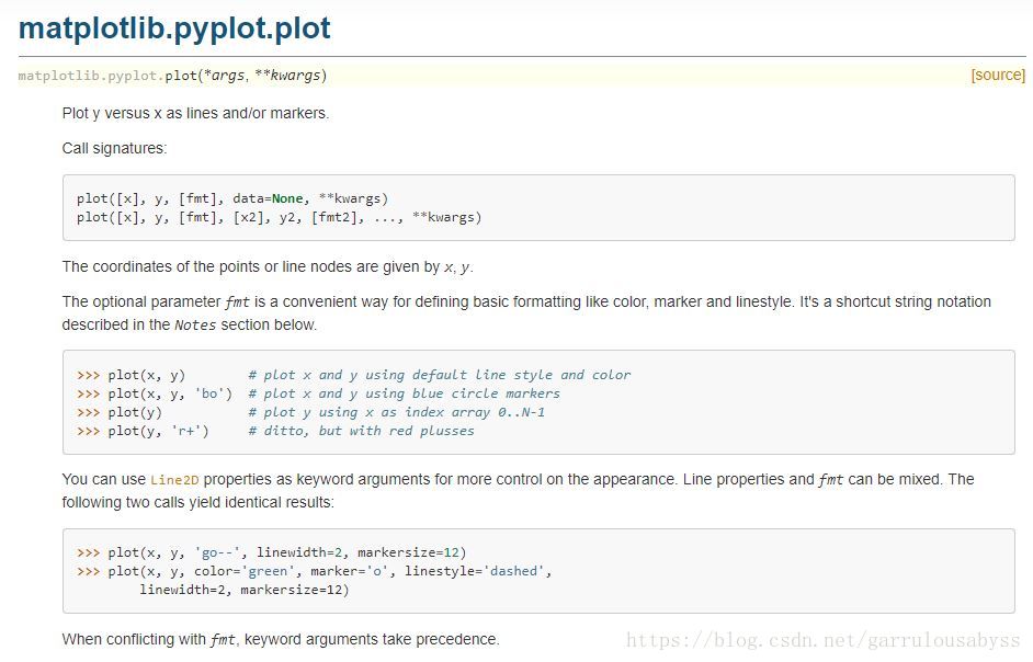
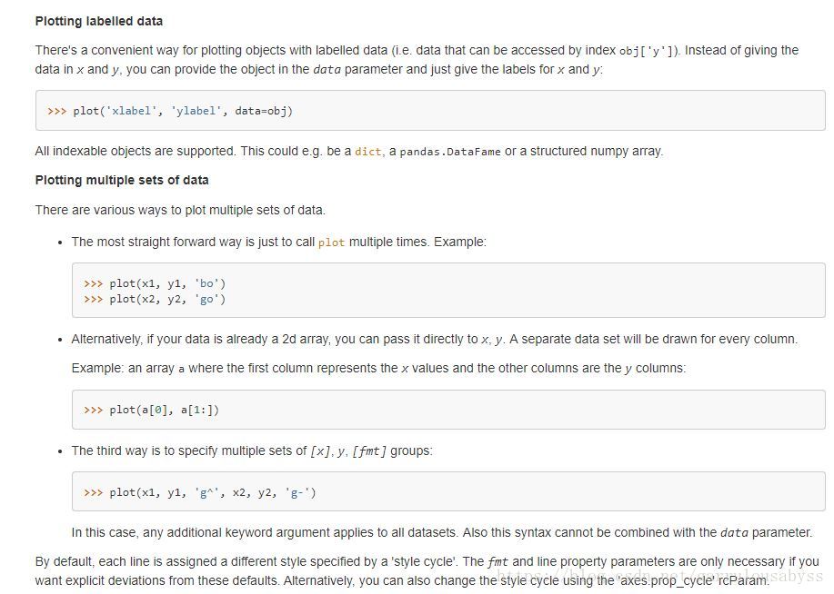
1. line plot

（1）首先要了解最基本的plot()函数相关的参数等，见下面两张图

接下来是一些常见图的代码及效果演示

import matplotlib
import matplotlib.pyplot as plt
import numpy as np

t = np.arange(0.0,2.0,0.01)
s = 1 + np.sin(2 * np.pi * t)

#Here use .subplots() to create multiple things in a graph.
#In other words, fig and ax are two different figs.
fig,ax = plt.subplots()

ax.plot(t,s)

ax.set(xlabel='time(s)',ylabel='voltage(mV)',title='About as simple as it gets, folks')
ax.grid()

fig.savefig('test.png')
plt.show()

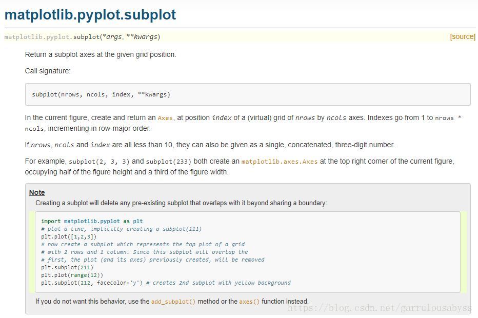
2. Multiple subplots in one figure

这里的话，首先要了解.subplot()函数

扫描二维码关注公众号，回复： 3038080 查看本文章

import numpy as np
import matplotlib.pyplot as plt

x1 = np.linspace(0.0, 5.0)
x2 = np.linspace(0.0, 2.0)

y1 = np.cos(2 * np.pi * x1) * np.exp(-x1)
y2 = np.cos(2 * np.pi * x2)

plt.subplot(2, 1, 1)
plt.plot(x1, y1, 'o-')
plt.title('A tale of 2 subplots')
plt.ylabel('Damped oscillation')

plt.subplot(2, 1, 2)
plt.plot(x2, y2, '.-')
plt.title('time (s)')
plt.ylabel('Undamped')

plt.show()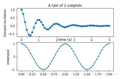

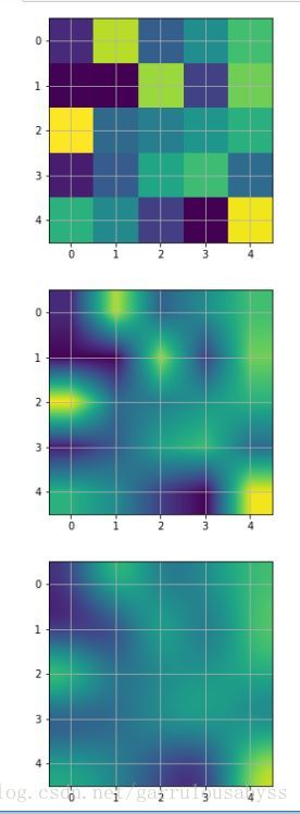
3.  Images

示例代码：

import matplotlib.pyplot as plt
import numpy as np

A = np.random.rand(5, 5)
plt.figure(1)
plt.imshow(A, interpolation='nearest')
plt.grid(True)

plt.figure(2)
plt.imshow(A, interpolation='bilinear')
plt.grid(True)

plt.figure(3)
plt.imshow(A, interpolation='bicubic')
plt.grid(True)

print(plt.show())

 

4. Contouring and pseudocolor