本周通过minist数据集的分类识别对softmax分类重新理解,终于理清了之前的迷惑。
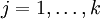
1、 softmax回归算法逻辑回归在多分类问题上的变体,我们知道线性回归解决的连续值的预测,逻辑回归解决的是离散值的预测,而且针对二分类问题。那么问题来了,如果是离散值预测,但是是多类别预测,也就是有多个类别标签,这种情况怎么办呢?Softmax回归针对的就是这种问题。
逻辑归回的假设函数如下:
逻辑回归的假设函数借用了sigmoid函数,而且逻辑回归中有一个假设上式代表取类别1的概率,而取类别0的概率我们用1-h(x)表示。在 softmax回归中,我们解决的是多分类问题,y可以取k个不同值,而并非只取两个值。因此,对于训练集 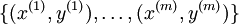 ,我们有
,我们有 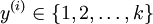 。(注意此处的类别下标从 1 开始,而不是 0)。对于给定的测试输入
  ,我们想用假设函数针对每一个类别j估算出概率值
  。也就是说,我们想估计 的每一种分类结果出现的概率。因此,我们的假设函数将要输出一个
  维的向量(向量元素的和为1)来表示这 个估计的概率值。 具体地说,我们的假设函数
  形式如下:
形式如下:
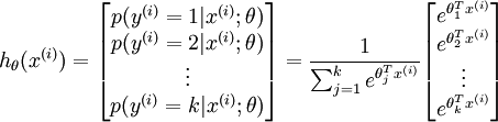
其中  是模型的参数。请注意
  这一项对概率分布进行归一化,使得所有概率之和为 1 (注意softmax函数与sigmoid函数并有什么关系)
个人注释:这里的模型参数其实是k个类型总共的模型参数,我们用逻辑回归的方法求解神经网络参数就是,每一个就是一个图片数据包括的全部的像素个数,例如一个28×28大小的图片数据拉成一个784的一维向量,如果有k个类别,则有个k×784个参数。然后通过上述公式对其进行归一化,使得输出各分类的概率之和为1。推广到深度神经网络是就是最后一层的处理方式。
2、代价函数有多种理解方式
先给出Softmax的函数形式如下:
![\begin{align}J(\theta) = - \frac{1}{m} \left[ \sum_{i=1}^{m} \sum_{j=1}^{k} 1\left\{y^{(i)} = j\right\} \log \frac{e^{\theta_j^T x^{(i)}}}{\sum_{l=1}^k e^{ \theta_l^T x^{(i)} }}\right]\end{align}](http://ufldl.stanford.edu/wiki/images/math/7/6/3/7634eb3b08dc003aa4591a95824d4fbd.png)
这个公式是怎么来的呢?我们可以从逻辑回归的代价函数推广而来。

![\begin{align}J(\theta) &= -\frac{1}{m} \left[ \sum_{i=1}^m (1-y^{(i)}) \log (1-h_\theta(x^{(i)})) + y^{(i)} \log h_\theta(x^{(i)}) \right] \\&= - \frac{1}{m} \left[ \sum_{i=1}^{m} \sum_{j=0}^{1} 1\left\{y^{(i)} = j\right\} \log p(y^{(i)} = j | x^{(i)} ; \theta) \right]\end{align}](http://ufldl.stanford.edu/wiki/images/math/5/4/9/5491271f19161f8ea6a6b2a82c83fc3a.png)
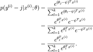
逻辑回归的代价函数是根据极大似然估计推理得来,Softmax的代价函数也类似。其实两个代价函数本质上一样的。我们可以把中括号中的加法看成,类别标签 × log(类别对应的概率),再累加。注意在Softmax回归中将 分类为类别 j的概率为:

在逻辑回归中我们梯度下降法求解最优值,Softmax回归也是用梯度下降法求解最优值,梯度公式如下:


3、Softmax回归模型参数具有“冗余”性
冗余性指的是最优解不止一个,有多个。假设我们从参数向量  中减去了向量
  ,这时,每一个 都变成了
  (
( )。此时假设函数变成了以下的式子:
我们看到,从 中减去 完全不影响假设函数的预测结果!这就是Softmax回归的冗余性。
4、Softmax回归与Logistic回归的关系
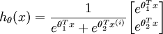
当类别数  时,softmax 回归退化为 logistic 回归。这表明 softmax 回归是 logistic 回归的一般形式。具体地说,当 时,softmax 回归的假设函数为:
利用softmax回归参数冗余的特点,我们令  ,并且从两个参数向量中都减去向量
  ,得到:
,得到:
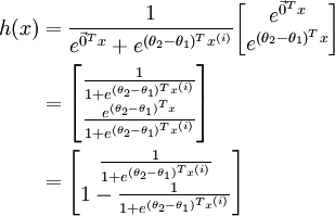
因此,用  来表示
来表示 ,我们就会发现 softmax 回归器预测其中一个类别的概率为
  ,另一个类别概率的为
 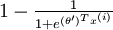 ,这与 logistic回归是一致的。
5、minist数据集及minist数据集逻辑回归分类任务程序
5.1程序:
import numpy as np
import tensorflow as tf
import matplotlib.pyplot as plt
from tensorflow.examples.tutorials.mnist import input_data
print ("大吉大利 今晚吃鸡")
#大吉大利 今晚吃鸡#
print ("下载中~别催了")
mnist = input_data.read_data_sets('data/', one_hot=True)
print
print (" 类型是 %s" % (type(mnist)))
print (" 训练数据有 %d" % (mnist.train.num_examples))
print (" 测试数据有 %d" % (mnist.test.num_examples))
#下载中~别催了#
#类型是 <class 'tensorflow.contrib.learn.python.learn.datasets.base.Datasets'>
训练数据有 55000
测试数据有 10000#
数据规格:
trainimg = mnist.train.images
trainlabel = mnist.train.labels
testimg = mnist.test.images
testlabel = mnist.test.labels
# 28 * 28 * 1
print (" 数据类型 is %s" % (type(trainimg)))
print (" 标签类型 %s" % (type(trainlabel)))
print (" 训练集的shape %s" % (trainimg.shape,))
print (" 训练集的标签的shape %s" % (trainlabel.shape,))
print (" 测试集的shape' is %s" % (testimg.shape,))
print (" 测试集的标签的shape %s" % (testlabel.shape,))
#数据类型 is <type 'numpy.ndarray'>
标签类型 <type 'numpy.ndarray'>
训练集的shape (55000, 784)
训练集的标签的shape (55000, 10)
测试集的shape' is (10000, 784)
测试集的标签的shape (10000, 10)#
看看数据集真面目:
看看庐山真面目
nsample = 5
randidx = np.random.randint(trainimg.shape[0], size=nsample)
for i in randidx:
curr_img = np.reshape(trainimg[i, :], (28, 28)) # 28 by 28 matrix
curr_label = np.argmax(trainlabel[i, :] ) # Label
plt.matshow(curr_img, cmap=plt.get_cmap('gray'))
print ("" + str(i) + "th 训练数据 "
+ "标签是 " + str(curr_label))
plt.show()
15932th 训练数据 标签是 4

49651th 训练数据 标签是 1


batch 数据
print ("Batch Learning? ")
batch_size = 100
batch_xs, batch_ys = mnist.train.next_batch(batch_size)
print ("Batch数据 %s" % (type(batch_xs)))
print ("Batch标签 %s" % (type(batch_ys)))
print ("Batch数据的shape %s" % (batch_xs.shape,))
print ("Batch标签的shape %s" % (batch_ys.shape,))
Batch Learning?
Batch数据 <type 'numpy.ndarray'>
Batch标签 <type 'numpy.ndarray'>
Batch数据的shape (100, 784)
Batch标签的shape (100, 10)
5.2
所需工具包
from tensorflow.examples.tutorials.mnist import input_data
import tensorflow as tf
mnist = input_data.read_data_sets('data/', one_hot=True)
设置参数:
numClasses = 10
inputSize = 784
trainingIterations = 50000
batchSize = 64
指定好x和y的大小
X = tf.placeholder(tf.float32, shape = [None, inputSize])
y = tf.placeholder(tf.float32, shape = [None, numClasses])
参数初始化
W1 = tf.Variable(tf.random_normal([inputSize, numClasses], stddev=0.1))
B1 = tf.Variable(tf.constant(0.1), [numClasses])
构造模型
y_pred = tf.nn.softmax(tf.matmul(X, W1) + B1)
loss = tf.reduce_mean(tf.square(y - y_pred))
opt = tf.train.GradientDescentOptimizer(learning_rate = .05).minimize(loss)
correct_prediction = tf.equal(tf.argmax(y_pred,1), tf.argmax(y,1))
accuracy = tf.reduce_mean(tf.cast(correct_prediction, "float"))
sess = tf.Session()
init = tf.global_variables_initializer()
sess.run(init)
迭代计算
for i in range(trainingIterations):
batch = mnist.train.next_batch(batchSize)
batchInput = batch[0]
batchLabels = batch[1]
_, trainingLoss = sess.run([opt, loss], feed_dict={X: batchInput, y: batchLabels})
if i%1000 == 0:
train_accuracy = accuracy.eval(session=sess, feed_dict={X: batchInput, y: batchLabels})
print ("step %d, training accuracy %g"%(i, train_accuracy))
#step 0, training accuracy 0.03125
step 1000, training accuracy 0.375
step 2000, training accuracy 0.625
step 3000, training accuracy 0.78125
step 4000, training accuracy 0.828125
step 5000, training accuracy 0.765625
step 6000, training accuracy 0.875
step 7000, training accuracy 0.8125
step 8000, training accuracy 0.8125
step 9000, training accuracy 0.90625
step 10000, training accuracy 0.890625
step 11000, training accuracy 0.875
step 12000, training accuracy 0.796875
step 13000, training accuracy 0.890625
step 14000, training accuracy 0.921875
step 15000, training accuracy 0.90625
step 16000, training accuracy 0.8125
step 17000, training accuracy 0.859375
step 18000, training accuracy 0.890625
step 19000, training accuracy 0.9375
step 20000, training accuracy 0.875
step 21000, training accuracy 0.90625
step 22000, training accuracy 0.875
step 23000, training accuracy 0.875
step 24000, training accuracy 0.9375
step 25000, training accuracy 0.921875
step 26000, training accuracy 0.890625
step 27000, training accuracy 0.890625
step 28000, training accuracy 0.90625
step 29000, training accuracy 0.953125
step 30000, training accuracy 0.90625
step 31000, training accuracy 0.9375
step 32000, training accuracy 0.859375
step 33000, training accuracy 0.90625
step 34000, training accuracy 0.90625
step 35000, training accuracy 0.953125
step 36000, training accuracy 0.859375
step 37000, training accuracy 0.796875
step 38000, training accuracy 0.921875
step 39000, training accuracy 0.90625
step 40000, training accuracy 0.90625
step 41000, training accuracy 0.921875
step 42000, training accuracy 0.953125
step 43000, training accuracy 0.921875
step 44000, training accuracy 0.84375
step 45000, training accuracy 0.921875
step 46000, training accuracy 0.921875
step 47000, training accuracy 0.921875
step 48000, training accuracy 0.859375
step 49000, training accuracy 0.828125#
测试结果
batch = mnist.test.next_batch(batchSize)
testAccuracy = sess.run(accuracy, feed_dict={X: batch[0], y: batch[1]})
print ("test accuracy %g"%(testAccuracy))
#test accuracy 0.875#
项目结束
2018.8.26