《一个图像复原实例入门深度学习&TensorFlow—第六篇》构建网络

构建网络

1.网络介绍

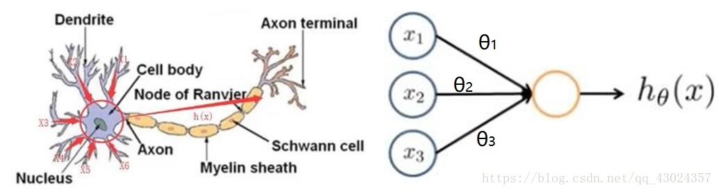
神经网络的原型受到人脑运作机制的启发，下图为一个神经细胞和神经网络中的一个神经元，神经细胞接收大量树突传递到过来的信号，然后神经细胞受到输入信号的刺激做出应激反应输出信号到轴突，轴突可以和其他神经元的树突相连，使得神经细胞之间能够交流信息。类似的，神经网络中的神经元也能接收其他神经元的输出，然后做出响应，响应的结果作为当前神经元的输出同时也是与之相连的下一个神经元的输入。
这里写图片描述
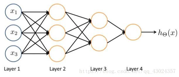
为了处理复杂问题，大脑中有很多很多神经细胞，来处理外界输入的复杂信息，并做出反应。同样的神经网络中也拥有大量神经元，信息通过神经元一层一层的传递，传递到最后得到一个输出结果，这个结果就是网络对输入信息的总体响应。
这里写图片描述
网络的结构对网络输出结果有巨大的影响，对于我们正在处理的这个图像复原的问题，我们选择应用效果最好的卷积神经网络。

2. 卷积神经网络

直接看这篇博文：https://blog.csdn.net/yunpiao123456/article/details/52437794
你要确保你知道下面的图的意思才继续往下看：
卷积：
这里写图片描述
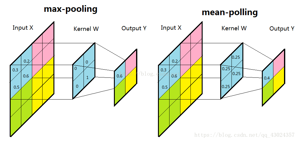
池化：

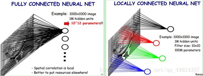
局部感知

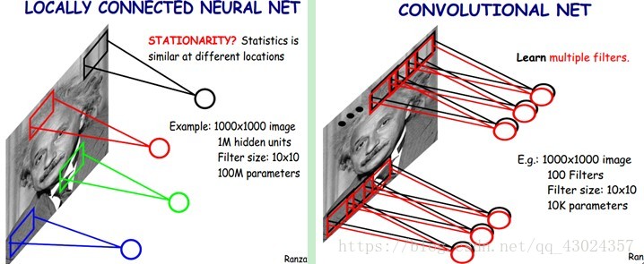
多核卷积

来，做两个题：
第一题：
输入层：图片28x28x1（长28 宽28 灰度图）
第一隐藏层（全连接）：784个节点
请问从输入层到第一隐藏层一共有多少个需要调整的连接权值？

28x28x1x784 + 784 = 615440

第一题：
输入层：图片28x28x1
第一隐藏层（卷积层）：卷积核大小：5x5 深度32
请问从输入层到第一隐藏层一共有多少个需要调整的连接权值？

5x5x1x32 + 32 = 832

3. 在TensorFlow中构建卷积神经网络

直接上核心代码：

# 定义权重的函数
def weight_variable(shape):
    initial = tf.truncated_normal(shape, stddev=0.1) # 从截断的正态分布中输出随机值μ-2σ，μ+2σ
    return tf.Variable(initial)
# 定义偏置的函数
def bias_variable(shape):
    initial = tf.constant(0.1, shape=shape)
    return tf.Variable(initial)
# 定义卷积层的函数
def conv2d(x, W):
    return tf.nn.conv2d(x, W, strides=[1, 1, 1, 1], padding='SAME')
# 定义池化层的函数
def max_pool_2x2(x):
    return tf.nn.max_pool(x, ksize=[1, 2, 2, 1],
                        strides=[1, 2, 2, 1], padding='SAME')        

# 定义将mini-batch导入网络的占位符
x = tf.placeholder(tf.float32, shape=[None,img_W,img_H,1],name = 'images')

# 第一卷积层
W_conv1 = weight_variable([5, 5, 1, 32])  
b_conv1 = bias_variable([32])
h_conv1 = tf.nn.relu(conv2d(x, W_conv1) + b_conv1)
# 第一池化层    
h_pool1 = max_pool_2x2(h_conv1)
# 第二卷积层
W_conv2 = weight_variable([5, 5, 32, 64])
b_conv2 = bias_variable([64])
h_conv2 = tf.nn.relu(conv2d(h_pool1, W_conv2) + b_conv2)
# 第二池化层      
h_pool2 = max_pool_2x2(h_conv2)
# 上采样层1        
W_de_conv1 = W_conv2
h_de_conv1 = tf.nn.conv2d_transpose(h_pool2,W_de_conv1,output_shape=[batch_size, 14, 14, 32],strides=[1,2,2,1],padding="SAME")
# 上采样层2
W_de_conv2 = W_conv1
h_de_conv2 = tf.nn.conv2d_transpose(h_de_conv1,W_de_conv2,output_shape=[batch_size, 28, 28, 1],strides=[1,2,2,1],padding="SAME")
# 网络输出的结果    
y_conv = h_de_conv2

这里特别说明一下：
1、卷积层的卷积核 W=[Filter_H，Filter_W，Input_Channels，Output_Channels ]，对于第一卷积层，我们定义了W_conv1 = weight_variable([5, 5, 1, 32])，也就是说卷积核的大小为5x5，上一层的图片数量为1，通过32个不同的卷积核（多核卷积）卷积得到32张不同的特征图。
2、由于池化层的存在，而且我们设置的卷积过程不改变图片的尺寸（strides=[1, 1, 1, 1], padding=’SAME’），所以经过两次池化后（根据设置的参数，一次池化图像缩小一倍），图片尺寸由28x28变为7x7，就我们手头要处理的图像复原问题，我们希望最后输出网络的图片和输入图片的尺寸相同，因此我们需要将图片进行两次上采样，这里用到函数：tf.nn.conv2d_transpose(h_pool2,W_de_conv1,output_shape=[batch_size, 14, 14, 32],strides=[1,2,2,1]，padding=”SAME”)，其中h_pool2是两次池化后输出的7x7的图片，W_de_conv1的shape是[5, 5, 32, 64]（[Filter_H，Filter_W，Output_Channels，Input_Channels]），output_shape=[batch_size, 14, 14, 32]（也就是第二池化之前的shape）strides=[1,2,2,1]（长x2 宽x2）padding=”SAME”（零填充）

4. 总结

本节构建卷积神经网络，虽然比较简略，但是结合提供的资源还有之前推荐的网易云吴恩达的公开课的第9章应该能很好的理解我们的卷积神经网络了。然后就是读懂代码了，实际我们在用的时候就是根据需求改一下矩阵的shape就好了，加多少层卷积层、池化层都大同小异。下面将之前的数据读取操作加进来，将mini-batch送入我们构建好的卷积神经网络，然后观察输出的网络的输出，代码如下：

import tensorflow as tf
import numpy as np
import matplotlib.pyplot as plt
from PIL import Image
import os

image_path = 'E:\\MNIST_data\\train_images\\'                # 输入图像的路径
label_path = 'E:\\MNIST_data\\train_labels\\'                # 输出图像的路径
TFRecord_path = 'E:\\MNIST_data\\tfrecord\\train_data_set.tfrecord'# 输出TFRecord文件的路径

img_W = 28      # 图像宽度
img_H = 28      # 图像高度
batch_size = 10 # 每个mini-batch含有的样本数量
min_after_dequeue = 1000 # 队列中最少文件数量
capacity = min_after_dequeue + 3*batch_size # 队列中最多文件数量

def _bytes_feature(value): # 生成字符串型的属性，用于存储图片像素信息，根据自己问题的要求选择要存的属性
     return tf.train.Feature(bytes_list=tf.train.BytesList(value=[value]))

# 将image_path和label_path中的图片一一对应封装在TFRecord_path中
def generate_TFRecordfile(image_path,label_path,TFRecord_path):
    images = []
    labels = []
    for file in os.listdir(image_path):
        images.append(image_path+file) # 得到所有转置图像的文件名
    for file in os.listdir(label_path):
        labels.append(label_path+file) # 得到所有未转置图像的文件名
    num_examples = len(images)         # 统计有多少用于训练的图片
    print('There are %d images for training\n'%(num_examples))

    writer = tf.python_io.TFRecordWriter(TFRecord_path) #创建一个writer写TFRecord文件
    for index in range(num_examples):
        print(index)
        image = Image.open(images[index]) # 打开一个image
        image = image.tobytes()           # 转换为字符型格式（因为之前生成的也是字符串型的属性嘛）
        label = Image.open(labels[index]) # 打开一个对应的label
        label = label.tobytes()           # 转换为字符型格式（因为之前生成的也是字符串型的属性嘛）
        #将一个样例转换为Example Protocol Buffer的格式，并且一组数据的信息都写入这个数据结构中,(打包咯)
        example = tf.train.Example(features=tf.train.Features(feature={
            'image':_bytes_feature(image),
            'label':_bytes_feature(label)}))
        writer.write(example.SerializeToString())#将这个example 写入TFRecord文件
    print('TFRecord file was generated successfully\n')
    writer.close()

def get_batch(TFRecord_path):
    reader = tf.TFRecordReader() # 创建一个reader来读取TFRecord文件中的样例 
    files = tf.train.match_filenames_once(TFRecord_path) # 获取文件列表
    # 创建文件名队列，乱序，每个样本使用num_epochs次
    filename_queue = tf.train.string_input_producer(files,shuffle = True,num_epochs = 1) 

    # 读取并解析一个样本
    _,example = reader.read(filename_queue)
    features = tf.parse_single_example(
        example,
        features={
            'image':tf.FixedLenFeature([],tf.string),
            'label':tf.FixedLenFeature([],tf.string)})

    # 使用tf.decode_raw将字符串解析成图像对应的像素数组 （）
    images = tf.decode_raw(features['image'],tf.uint8)
    labels = tf.decode_raw(features['label'],tf.uint8)

    # 所得像素数组为shape为(（img_W*img_H）,)，应该reshape
    images = tf.reshape(images, shape=[img_W,img_H])
    labels = tf.reshape(labels, shape=[img_W,img_H])

    #在这里添加图像预处理函数（optional）

    #使用tf.train.shuffle_batch来随机组合数据生成用于随机梯度下降的mini-batch
    Image_Batch,Label_Batch = tf.train.shuffle_batch([images,labels],
                                             batch_size = batch_size,
                                             num_threads = 5,
                                             min_after_dequeue = min_after_dequeue,
                                             capacity = capacity)
    return Image_Batch,Label_Batch

    # 定义权重的函数
def weight_variable(shape):
    initial = tf.truncated_normal(shape, stddev=0.1) # 从截断的正态分布中输出随机值μ-2σ，μ+2σ
    return tf.Variable(initial)
    # 定义偏置的函数
def bias_variable(shape):
    initial = tf.constant(0.1, shape=shape)
    return tf.Variable(initial)
    # 定义卷积层的函数
def conv2d(x, W):
    return tf.nn.conv2d(x, W, strides=[1, 1, 1, 1], padding='SAME')
    # 定义池化层的函数
def max_pool_2x2(x):
    return tf.nn.max_pool(x, ksize=[1, 2, 2, 1],
                            strides=[1, 2, 2, 1], padding='SAME')        
generate_TFRecordfile(image_path,label_path,TFRecord_path) # 调用函数生成TFRecord文件
Image_Batch,Label_Batch = get_batch(TFRecord_path)   # 调用函数多线程读取TFRecord文件生成mini-batch       
# 定义将mini-batch导入网络的占位符
x = tf.placeholder(tf.float32, shape=[None,img_W,img_H,1],name = 'images')

# 第一卷积层
W_conv1 = weight_variable([5, 5, 1, 32])  
b_conv1 = bias_variable([32])
h_conv1 = tf.nn.relu(conv2d(x, W_conv1) + b_conv1)
# 第一池化层    
h_pool1 = max_pool_2x2(h_conv1)
# 第二卷积层
W_conv2 = weight_variable([5, 5, 32, 64])
b_conv2 = bias_variable([64])
h_conv2 = tf.nn.relu(conv2d(h_pool1, W_conv2) + b_conv2)
# 第二池化层      
h_pool2 = max_pool_2x2(h_conv2)
# 上采样层1        
W_de_conv1 = W_conv2
h_de_conv1 = tf.nn.conv2d_transpose(h_pool2,W_de_conv1,output_shape=[batch_size, 14, 14, 32],strides=[1,2,2,1],padding="SAME")
# 上采样层2
W_de_conv2 = W_conv1
h_de_conv2 = tf.nn.conv2d_transpose(h_de_conv1,W_de_conv2,output_shape=[batch_size, 28, 28, 1],strides=[1,2,2,1],padding="SAME")
# 网络输出的结果    
y_conv = h_de_conv2

init_op = (tf.local_variables_initializer(),tf.global_variables_initializer())#初始化操作
with tf.Session() as sess:
    sess.run(init_op)
    coord = tf.train.Coordinator() # 用于协调多个线程同时终止
    threads = tf.train.start_queue_runners(sess=sess,coord=coord) # 启动线程
    try:
        for step in range(5500):
            if coord.should_stop(): # 读到结束标记后coord.should_stop()变为True，跳出循环
                break
            image_batch,label_batch = sess.run([Image_Batch,Label_Batch])# 得到一个mini-batch
            image_batch = np.reshape(image_batch,[batch_size,img_W,img_H,1]) # 一个样本为行
            label_batch = np.reshape(label_batch,[batch_size,img_W,img_H,1])
            #将mini-batch通过占位符x送入网络，得到网络的输出结果
            y_pred = sess.run(y_conv,feed_dict={x:image_batch})# 得到一个mini-batch

        #画个图        
        input_img = image_batch[0,:,:] # 取一个mini-batch(10张)中的一张出来看看
        output_img = y_pred[0,:,:] 
        label = label_batch[0,:,:]       
        input_img = np.reshape(input_img,[28,28])
        output_img = np.reshape(output_img,[28,28])
        label = np.reshape(label,[28,28])      
        input_img = Image.fromarray(input_img.astype('uint8')).convert('L')
        output_img = Image.fromarray(output_img.astype('uint8')).convert('L')
        label = Image.fromarray(label.astype('uint8')).convert('L')        
        plt.imshow(input_img)
        plt.show() 
        plt.imshow(output_img)
        plt.show() 
        plt.imshow(label)
        plt.show()                  
    except tf.errors.OutOfRangeError: # 捕捉文件名队列中的结束标记
        print('epoch limit reached')
        coord.request_stop() #通知其它线程停止读取数据
    finally:
        coord.request_stop()
        coord.join(threads) #等待所有线程退出

复制代码到Spyder中，运行得到结果：
这里写图片描述
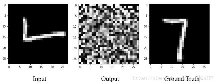
哇，什么鬼，网络根本就没用嘛！
我想你肯定知道为什么会得到这么不靠谱的结果，是的，我们根本没有训练网络，网络现在还属于只会瞎猜的状态。
下一节，我们将训练我们构建的卷积神经网络，让它变得聪明一些。