Sklearn--不平二分类交叉验证及模型评估指标选择

该篇侧重点在于不平二分类的评估指标选择

1、数据说明

数据为 MNIST 有70000张图片，每张图片有784个特征。
每个图片都是28*28像素的，并且每个像素的值介于0~255之间

2、模型训练

# 将数据集改为一个二分类的，分为5和非5
y_train_5 = (y_train == 5)
y_test_5 = (y_test == 5)

# 用SGDClassifier类（梯度下降分类器）。
from sklearn.linear_model import SGDClassifier
sgd_clf = SGDClassifier(random_state= 42) 
sgd_clf.fit(x_train, y_train_5)

# 查看预测情况
sgd_clf.predict([x_train[7000]])
y_train[7000]

SGDClassifier 依赖于训练集的随机程度,所以之前训练集用numpy.random.permutation 打乱过顺序

3、模型评估

3.1 精度评估

3.1.1分层采样交叉验证

from sklearn.model_selection import StratifiedKFold
from sklearn.base import clone

skfolds = StratifiedKFold(n_splits=3, random_state=42) # 分层采样
for train_index, test_index in skfolds.split(x_train, y_train_5):  # 分层采样索引
    clone_clf = clone(sgd_clf)  # 克隆分类器
    #### 提取分层采样数据
    x_train_folds = x_train[train_index]
    y_train_folds= y_train_5[train_index]
    x_test_folds = x_train[test_index]
    y_test_folds = y_train_5[test_index]
    #### 模型评估
    clone_clf.fit(x_train_folds, y_train_folds)
    y_pred = clone_clf.predict(x_test_folds)
    n_correct = sum(y_pred == y_test_folds)
    print(n_correct / len(y_pred)

3.1.2 简单的交叉验证

from sklearn.model_selection import cross_val_score
cross_val_score(sgd_clf, x_train, y_train_5, cv=3, scoring='accuracy')

模型的精度在 0.94 左右
但是实际上从sum(y_train_5)/len(y_train_5) 可以知道数字5仅仅占总的样本中的 0.09035
也就是说随便猜不是5 他的准确度也可以达到90%
所以精度这个指标不具有代表性

3.1.3 验证精度指标不具有代表性——用相当笨的分类去分

from sklearn.base import BaseEstimator
class Never5Classifier(BaseEstimator):
    def fit(self, x, y=None):
        pass
    def predict(self, x):
        return np.zeros((len(x), 1), dtype = bool)


never_5_clf = Never5Classifier()
cross_val_score(never_5_clf, x_train, y_train_5, cv=3, scoring='accuracy')
##  0.91105, 0.90995, 0.90795 约等于 1- 0.09035 = 0.90965

3.2 准确率和召回率

准确率和召回率，需要分类正确和错误的全部结果，可以从sklearn.model_selection的 cross_val_predict 中获得
然后和实际结果连列成混淆矩阵（sklearn.metrics）

可以看混淆矩阵

from sklearn.model_selection import cross_val_predict
y_train_pred = cross_val_predict(sgd_clf, x_train, y_train_5, cv=3)

from sklearn.metrics import confusion_matrix
confusion_matrix(y_train_5, y_train_pred)

# result 很明显 1118和3751这一列是 预测为5, 可见模型实际上是在预测不是5
array([[53461,  1118],
       [ 1670,  3751]], dtype=int64)

也可以直接看准确率和召回率

from sklearn.metrics import precision_score, recall_score, f1_score
precision_score = precision_score(y_train_5, y_train_pred)  # 0.7703840624358185
recall = recall_score(y_train_5, y_train_pred)              # 0.6919387566869581
f1 = f1_score(y_train_5, y_train_pred)                      # 0.7290573372206025

从该数据集来说召回率0.691，准确率0.770，并不理想。从算法角度分析，可以用改变阈值的方法改进模型，因此可以绘制曲线来选取适当阈值

1. 用decision_function()提取分数

y_scores = sgd_clf.decision_function([some_digit])
threshold = 0
y_some_digit_pred = (y_scores > threshold)

y_scores = cross_val_predict(sgd_clf, x_train, y_train_5, cv=3,
                             method = 'decision_function')

2. 计算不同阈值下的准确率和召回率，绘制图形

# 计算不同阈值下的准确率和召回率
from sklearn.metrics import precision_recall_curve  
precisions, recalls, thresholds = precision_recall_curve(y_train_5, y_scores)

# 绘制图形
import matplotlib.pyplot as plt
plt.style.use('ggplot')

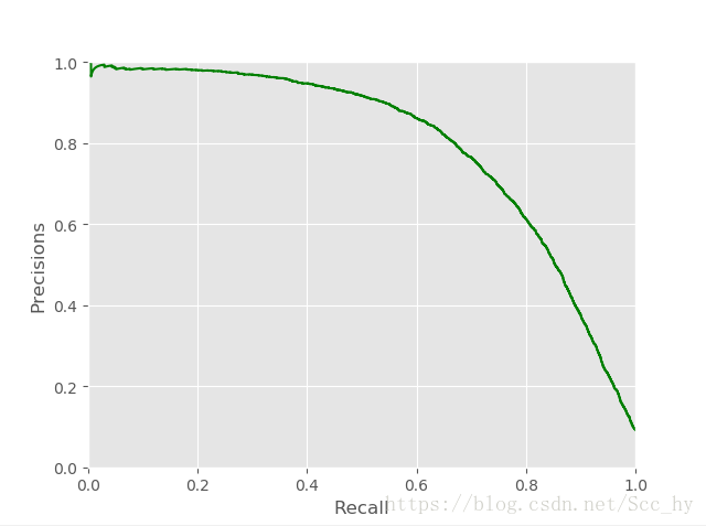
## 召回率和准确率曲线
plt.plot(recalls[:-1], precisions[:-1], 'g-')
plt.xlim(0, 1)
plt.ylim(0, 1)
plt.xlabel('Recall')
plt.ylabel('Precisions')
plt.show()
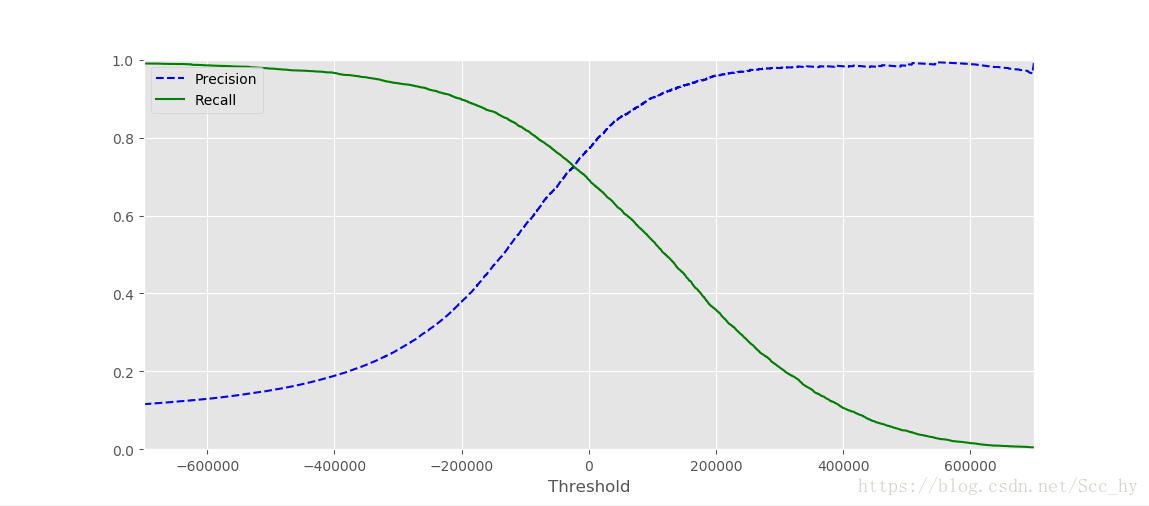
## 阈值和召回率与准确率曲线
plt.plot(thresholds, precisions[:-1],'b--',label='Precision')
plt.plot(thresholds, recalls[:-1], 'g-', label='Recall')
plt.xlabel('Threshold')
plt.legend(loc='upper left')
plt.ylim(0,1)
plt.xlim(-700000, 700000)
plt.show()

recall 0.8 左右的时候，准确率急剧下降。优先考虑准确率的时候可以在recall 0.6的时候选一个点，且这时候准确率也接近0.9
这里写图片描述

从上图确定recall0.6左右，precision 0.9左右，因此从下图中可以取阈值65000
这里写图片描述

from sklearn.metrics import precision_score, recall_score
y_train_pred_90 = (y_scores > 65000)

precision_score(y_train_5, y_train_pred_90)  # 0.8672781224710008
recall_score(y_train_5, y_train_pred_90)     # 0.5930640103301974

3.3 ROC曲线和AUC

# ROC曲线
from sklearn.metrics import roc_curve
fpr, tpr, thresholds = roc_curve(y_train_5, y_scores) #需要正确分类和预测值，进行阈值逐步调整

def plot_roc_curve(fpr, tpr, label=None):
    plt.plot(fpr, tpr, lw=2, label = label)
    plt.plot([0,1],[0,1],'k--')
    plt.axis([0, 1, 0, 1])
    plt.xlabel('False Positive Rate') # 特异度 True Negative rate
    plt.ylabel('True Positive Rate')  # 召回率

plot_roc_curve(fpr, tpr)
plt.show()

# AUC 的值
from sklearn.metrics import roc_auc_score
roc_auc_score(y_train_5, y_scores)          # 默认阈值 0.946327917941239
roc_auc_score(y_train_pred_90, y_scores)    # 调整阈值 1.0
## 可见AUC值在不平分类的时候作为模型评估不是十分恰当

因为ROC曲线和准确率/召回率曲线（PR）很类似，
笨拙的规则曲线选择：当正例很少，或者你关注假正例多余假反例的时候：优先使用PR曲线
其他情况使用ROC曲线