机器学习笔记--TensorFlow学习笔记(4)--MNIST机器学习深入

使用神经网络识别MNIST数据集
总代码：
#!/usr/bin/env python
# -*- coding: utf-8 -*-
'使用MNIST 进行手写数字识别_构建一个多层卷积网络'

# 0.导入
# 使用tensorflow之前，首先导入它
import tensorflow as tf
# 导入mnist数据
from tensorflow.examples.tutorials.mnist import input_data
mnist=input_data.read_data_sets('MNIST_data',one_hot=True)
sess = tf.InteractiveSession()
# 使用InteractiveSession类可以更加灵活地构建代码：在运行图的时候，插入一些计算图，这些计算图是由某些操作(operations)构成的。
# 如果没有使用InteractiveSession，那么需要在启动session之前构建整个计算图，然后启动该计算图。


# 1.占位符和变量
x = tf.placeholder("float", shape = [None, 784])
y_ = tf.placeholder("float", shape = [None, 10])

W = tf.Variable(tf.zeros([784, 10]))
b = tf.Variable(tf.zeros([10]))

# 我们需创建大量的权重和偏置项，权重在初始化时应加入少量噪声打破对称性以及避免0梯度
# 使用的是RELU神经元，比较好的做法是用一个较小的正数来初始化偏置项，以避免神经元节点输出恒为0的问题(dead neurons)
def weight_variable(shape):
    initial = tf.truncated_normal(shape, stddev = 0.1)
    return tf.Variable(initial)

def bias_variable(shape):
    initial = tf.constant(0.1, shape = shape)
    return tf.Variable(initial)

# 2.建立模型
# 2.0 卷积和池化
# 卷积使用1步长(stride size)，0边距(padding size)的模板，保证输出和输入是同一个大小
# conv2d设置可看这里：https://github.com/jikexueyuanwiki/tensorflow-zh/blob/master/SOURCE/api_docs/python/nn.md#conv2d
def conv2d(x, W):
    return tf.nn.conv2d(x, W,strides = [1, 1, 1, 1], padding = 'SAME')
# 池化用简单传统的2x2大小的模板做max pooling
def max_pool_2x2(x):
    return tf.nn.max_pool(x, ksize = [1, 2, 2, 1], strides = [1, 2, 2, 1], padding = 'SAME')

# 2.1 第一层卷积：由一个卷积接一个max pooling完成
# 卷积在每个5x5的patch中算出32个特征，卷积的权重张量形状是[5, 5, 1, 32]，前两个维度是patch的大小，
# 接着是输入的通道数目，最后是输出的通道数目。而对于每一个输出通道都有一个对应的偏置量。
W_conv1 = weight_variable([5, 5, 1, 32])
b_conv1 = bias_variable([32])
# 为了用这一层，把x变成一个4d向量，其第2、第3维对应图片的宽、高，最后一维代表图片的颜色通道数
# (因为是灰度图所以这里的通道数为1，如果是rgb彩色图，则为3)。
x_image = tf.reshape(x, [-1, 28, 28, 1])
# 我们把x_image和权值向量进行卷积，加上偏置项，然后应用ReLU激活函数，最后进行max pooling。
h_conv1 = tf.nn.relu(conv2d(x_image, W_conv1) + b_conv1)
h_pool1 = max_pool_2x2(h_conv1)

# 2.2 第二层卷积
# 为了构建一个更深的网络，我们会把几个类似的层堆叠起来。第二层中，每个5x5的patch会得到64个特征。
W_conv2 = weight_variable([5, 5, 32, 64])
b_conv2 = bias_variable([64])

h_conv2 = tf.nn.relu(conv2d(h_pool1, W_conv2) + b_conv2)
h_pool2 = max_pool_2x2(h_conv2)


# 2.3 密集连接层
# 现在，图片尺寸减小到7x7，我们加入一个有1024个神经元的全连接层，用于处理整个图片。
# 我们把池化层输出的张量reshape成一些向量，乘上权重矩阵，加上偏置，然后对其使用ReLU。
W_fc1 = weight_variable([7 * 7 * 64, 1024])
b_fc1 = bias_variable([1024])

h_pool2_flat = tf.reshape(h_pool2, [-1, 7 * 7 * 64])
h_fc1 = tf.nn.relu(tf.matmul(h_pool2_flat, W_fc1) + b_fc1)


# 2.4 Dropout
# 为减少过拟合，在输出层之前加入dropout
keep_prob = tf.placeholder("float")
h_fc1_drop = tf.nn.dropout(h_fc1, keep_prob)


# 2.5 输出层
W_fc2 = weight_variable([1024, 10])
b_fc2 = bias_variable([10])

y_conv = tf.nn.softmax(tf.matmul(h_fc1_drop, W_fc2) + b_fc2)


# 3.训练和评估模型
# 使用更加复杂的ADAM优化器来做梯度最速下降
# 在feed_dict中加入额外的参数keep_prob来控制dropout比例。然后每100次迭代输出一次日志。
cross_entropy = -tf.reduce_sum(y_*tf.log(y_conv))
train_step = tf.train.AdamOptimizer(1e-4).minimize(cross_entropy)
correct_prediction = tf.equal(tf.argmax(y_conv, 1), tf.argmax(y_, 1))
accuracy = tf.reduce_mean(tf.cast(correct_prediction, "float"))


init = tf.initialize_all_variables()
sess.run(init)

for i in range(5000):
    batch = mnist.train.next_batch(50)
    if i % 100 == 0:
        train_accuracy = accuracy.eval(feed_dict = {x: batch[0], y_: batch[1], keep_prob: 1.0})
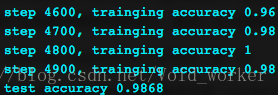
        print("step %d, trainging accuracy %g" %(i, train_accuracy))
    train_step.run(feed_dict = {x: batch[0], y_: batch[1], keep_prob: 0.5})

print("test accuracy %g" %accuracy.eval(feed_dict = {x: mnist.test.images, y_: mnist.test.labels, keep_prob: 1.0}))
上面的代码中训练了5000次，教程里给的是20000次，训练结果：
这里写图片描述
机器学习笔记--TensorFlow学习笔记(4)--MNIST机器学习深入

猜你喜欢
