数据分析中篇（数据清洗&特征处理常见手法）

数据裁剪、压缩、累乘

ndarray.clip(min=最小值, max=最大值)
将调用数组中小于min的元素设置为min，大于max的元素设置为max。
ndarray.compress(条件)
返回调用数组中满足给定条件的元素。
ndarray.prod()
返回调用数组中各元素的乘积。
ndarray.cumprod()
返回调用数组中各元素计算累乘的过程数组。

import numpy as np

a = np.arange(1,10).reshape(3,3)
print("a---------")
print(a)
b = a.clip(min = 3,max = 7)
print("b---------")
print(b)


c = a.compress(a.ravel()<7).reshape(-1,3)
print("-c--------")
print(c)


f = a.prod()
print("f---------")
print(f)
g = 1
for elem in a.flat:
    g*=elem
print("g---------")
print(g)
h = a.cumprod()
print("h---------")
print(h)

数据相关性计算

使用模块 numpy
numpy.corrcoef(a, b)->相关性矩阵
corr = np.corrcoef(bhp_returns,vale_returns)

import  datetime as dt
import numpy as np
import matplotlib.pyplot as mp
import matplotlib.dates as md


def dmy2day(dmy):

    '''
    文件中的日期转化为星期
    :param dmy:
    :return:
    '''
    dmy = str(dmy,encoding='utf-8')
    date = dt.datetime.strptime(dmy,'%d-%m-%Y').date()
    wday = date.weekday()
    ymd = date.strftime('%Y-%m-%d')

    return ymd
dates,bhp_closing_price=np.loadtxt("bhp.csv",
                                    delimiter=',',
                                    usecols=(1,6),
                                    unpack=True,
                                    dtype=np.dtype('M8[D],f8'),
                                    converters={1:dmy2day},
                                    )
_,vale_closing_price=np.loadtxt("vale.csv",
                                 delimiter=',',
                                 usecols=(1,6),
                                 unpack=True,
                                 dtype=np.dtype('M8[D],f8'),
                                 converters={1:dmy2day},
                                  )
bhp_returns= np.diff(bhp_closing_price)/bhp_closing_price[:-1]  #后一列减去前一列的差
vale_returns= np.diff(vale_closing_price)/vale_closing_price[:-1]
corr = np.corrcoef(bhp_returns,vale_returns)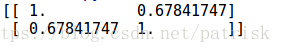

矢量化

对numpy数组进行多次运算
def 标量函数(标量参数1, 标量参数2, ...):
...
return 标量返回值1, 标量返回值2, ...
np.vectorize(标量函数)->矢量函数

def fun(a, b):
    return a + b, a - b, a * b
A = np.array([10, 20, 30])
B = np.array([100, 200, 300])
C = np.vectorize(fun)(A, B)
print(C)

数据平滑&卷积降噪

卷积

卷积过程
a:[1 2 3 4 5]---被卷积数组
b:[6 7 8]----卷积核数组
卷积过程：
b先按中心7旋转180°形成b` = [8 7 6]
b`按照a的方向遍历a，对应位置相乘且相加，
a对应的位置没有元素一般采用0补齐
下面是起始遍历位置和终止遍历位置
  0 0 1 2 3 4 5
  8 7 6
  8*0+7*0+1*6 = 6
  0 0 1 2 3 4 5 0 0
              8 7 6
  8*5+7*0+6*0 = 40
   卷积计算结果如下
   full：6  19  40  61  82   67  40
   same：19 40 61 82 67
   valid：40 61 82
   其中full代表：卷积结果的大小与补全后的大小相同
   same代表：卷积结果与a原本的大小相同
   vaild 代表：卷积结果与核向量相同
 计算函数
   numpy.convolve(a,b,'full/'same'/valid)

import numpy as np
a = np.arange(1, 6)
print('a:', a)
b = np.arange(6, 9)
print('b:', b)
c = np.convolve(a, b, 'full')
print('c ( full):', c)
c = np.convolve(a, b, 'same')
print('c ( same):', c)
c = np.convolve(a, b, 'valid')
print('c (valid):', c)

数据平滑函数

对于非周期的连续数u，在对其进行卷积降噪时可以采用汉宁函数产生
其卷积核矩阵，对数据进行平滑
N：窗口大小，可以自己设定
weight= np.hanning(N)
c = np.convolve(array,weights,'valid')

import datetime as dt
import numpy as np
import matplotlib.pyplot as mp
import matplotlib.dates as md

def dmy2ymd(dmy):
    dmy = str(dmy, encoding='utf-8')
    date = dt.datetime.strptime(
        dmy, '%d-%m-%Y').date()
    ymd = date.strftime('%Y-%m-%d')
    return ymd
dates, bhp_closing_prices = np.loadtxt(
    'bhp.csv', delimiter=',',
    usecols=(1, 6), unpack=True,
    dtype=np.dtype('M8[D], f8'),
    converters={1: dmy2ymd})
_, vale_closing_prices = np.loadtxt(
    'vale.csv', delimiter=',',
    usecols=(1, 6), unpack=True,
    dtype=np.dtype('M8[D], f8'),
    converters={1: dmy2ymd})


bhp_returns = np.diff(
    bhp_closing_prices) / bhp_closing_prices[:-1]
vale_returns = np.diff(
    vale_closing_prices) / vale_closing_prices[:-1]
N = 8
weights = np.hanning(N)  # 汉宁窗
weights /= weights.sum()


bhp_smooth_returns = np.convolve(
    bhp_returns, weights, 'valid')
vale_smooth_returns = np.convolve(
    vale_returns, weights, 'valid')
mp.figure('Smoothing Returns',
          facecolor='lightgray')
mp.title('Smoothing Returns', fontsize=20)
mp.xlabel('Date', fontsize=14)
mp.ylabel('Returns', fontsize=14)
ax = mp.gca()
ax.xaxis.set_major_locator(
    md.WeekdayLocator(byweekday=md.MO))
ax.xaxis.set_minor_locator(
    md.DayLocator())
ax.xaxis.set_major_formatter(
    md.DateFormatter('%d %b %Y'))
mp.tick_params(labelsize=10)
mp.grid(linestyle=':')
dates = dates.astype(md.datetime.datetime)
mp.plot(dates[:-1], bhp_returns, c='orangered',
        alpha=0.25, label='BHP')
mp.plot(dates[:-1], vale_returns, c='dodgerblue',
        alpha=0.25, label='VALE')
mp.plot(dates[N - 1:-1], bhp_smooth_returns,
        c='orangered', alpha=0.75,
        label='Smooth BHP')
mp.plot(dates[N - 1:-1], vale_smooth_returns,
        c='dodgerblue', alpha=0.75,
        label='Smooth VALE')
dates, returns = np.hsplit(inters, 2)
dates = dates.astype(int).astype(
    'M8[D]').astype(md.datetime.datetime)
mp.scatter(dates, returns, marker='x',
           c='firebrick', s=100, lw=3, zorder=3)
mp.legend()
mp.gcf().autofmt_xdate()
mp.show()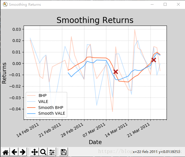

数组插入&排序&插值处理

np.lexsort((参考序列，待排序列)) 返回索引序列
np.searchsorted(有序序列，被插序列)返回插入位置
np.insert(有序序列，插入位置，被插序列)返回插入结果
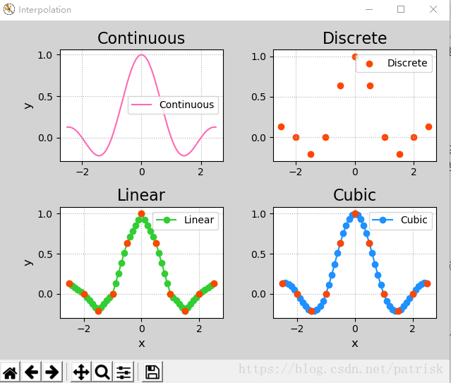
import scipy.interpolate as si
si.interp1d(离散样本水平坐标，离散样本垂直坐标,
kind=插值器种类)->一维插值器对象

# -*- coding: utf-8 -*-
from __future__ import unicode_literals
import numpy as np
import scipy.interpolate as si
import matplotlib.pyplot as mp
min_x, max_x = -2.5, 2.5
con_x = np.linspace(min_x, max_x, 1001)
con_y = np.sinc(con_x)
dis_x = np.linspace(min_x, max_x, 11)
dis_y = np.sinc(dis_x)
linear = si.interp1d(dis_x, dis_y)
lin_x = np.linspace(min_x, max_x, 51)
lin_y = linear(lin_x)
cubic = si.interp1d(dis_x, dis_y, kind='cubic')
cub_x = np.linspace(min_x, max_x, 51)
cub_y = cubic(cub_x)
mp.figure('Interpolation', facecolor='lightgray')
mp.subplot(221)
mp.title('Continuous', fontsize=16)
mp.ylabel('y', fontsize=12)
mp.tick_params(labelsize=10)
mp.grid(linestyle=':')
mp.plot(con_x, con_y, c='hotpink',
        label='Continuous')
mp.legend()
mp.subplot(222)
mp.title('Discrete', fontsize=16)
mp.tick_params(labelsize=10)
mp.grid(linestyle=':')
mp.scatter(dis_x, dis_y, c='orangered',
           label='Discrete')
mp.legend()
mp.subplot(223)
mp.title('Linear', fontsize=16)
mp.xlabel('x', fontsize=12)
mp.ylabel('y', fontsize=12)
mp.tick_params(labelsize=10)
mp.grid(linestyle=':')
mp.plot(lin_x, lin_y, 'o-', c='limegreen',
        label='Linear')
mp.scatter(dis_x, dis_y, c='orangered', zorder=3)
mp.legend()
mp.subplot(224)
mp.title('Cubic', fontsize=16)
mp.xlabel('x', fontsize=12)
mp.tick_params(labelsize=10)
mp.grid(linestyle=':')
mp.plot(cub_x, cub_y, 'o-', c='dodgerblue',
        label='Cubic')
mp.scatter(dis_x, dis_y, c='orangered', zorder=3)
mp.legend()
mp.tight_layout()
mp.show()

一些常用的小函数

np.isreal(obj)    #判断obj是否是全实数的矩阵
np.diff(numpy.col)   #数组的前前一列减去后一列
np.matrix(可被解释为矩阵的容器，copy=[True/False])
np.mat(可被解释为矩阵的二维容器，数据共享，相当于copy=False的matix())
np.add.reduce(数组)#对数组进行累加
np.add.accumulate(数组)   #显示累加过程
np.add.reduceat(数组,[位置])  #在指定位置累加
np.floor_divide()     #天花板除，即结果取大于结果的
np.ceil()             #地板除，即结果取小于
np.trunc()            #截断除，即结果只要整数部分

整理的时候突然发现有个人整理的更棒传送门此处烂笔头numpy使用笔记

a = np.arange(1,7)
d = np.add.reduceat(a, [0, 2, 4])
1 2 3 4 5 6 
0   2   4
  3   7   11