人工智能实践： 卷积神经网络实践

复现已有的卷积神经网络

VGGNet是Karen simonyan等人在2015年的ICLR会议中，公开的神经网络模型。这个模型在2014年的ImageNet比赛中获得了定位第一名和分类第二名的成绩。论文为VeryDeep Convolutional Networks for Large-Scale Image Recognition，这篇博客对该论文介绍的非常详细。这篇文章是以比赛为目的——解决ImageNet中的1000类图像分类和localization。作者对六个网络的实验结果在深度对模型影响方面，进行了感性分析（越深越好），实验结果是16和19层的VGGNet（VGG代表了牛津大学的Oxford Visual Geometry Group，该小组隶属于1985年成立的Robotics Research Group，该Group研究范围包括了机器学习到移动机器人）分类和localization的效果好。

VGG实现代码重点讲解  

x = tf.placeholder(tf.float32,shape =[BATCH_SIZE,IMAGE_PIXELS])

tf.placeholder：用于传入真实训练样本/ 测试/ 真实特征/ 待处理特征。只是占位，不必给出初值。

用sess.run的feed_dict参数以字典形式喂入x:, y_: sess.run(feed_dict = {x: ,y_: })

BATCH_SIZE：一次传入的个数。 IMAGE_PIXELS：图像像素。

例：x = tf.placeholder("float",[1,224,224,3])

BATCH_SIZE为1，表示一次传入一个。图像像素为[224,224,3]。

w =tf.Variable(tf.random_normal())：从正态分布中给出权重w的随机值。   

b = tf.Variable(tf.zeros())：统一将偏置b初始化为0。

注意：以上两行函数Variable中的V要大写，Variable必须给初值。

np.load  np.save:将数组以二进制格式保存到磁盘，扩展名为.npy 。

.item()：遍历（键值对）。

tf.shape(a)和a.get_shape()比较

相同点：都可以得到tensor a的尺寸     

不同点：tf.shape()中 a 的数据类型可以是 tensor, list, array；

而a.get_shape()中a的数据类型只能是tensor,且返回的是一个元组（tuple）。

例：

import tensorflow as tf     

import numpy as np

x=tf.constant([[1,2,3],[4,5,6]]   

y=[[1,2,3],[4,5,6]]    

z=np.arange(24).reshape([2,3,4]))

sess=tf.Session()     #tf.shape()     

x_shape=tf.shape(x)          

# x_shape 是一个tensor     

y_shape=tf.shape(y)          # <tf.Tensor 'Shape_2:0' shape=(2,) dtype=int32>    

z_shape=tf.shape(z)         #  <tf.Tensor 'Shape_5:0'shape=(3,) dtype=int32>     

print sess.run(x_shape)      # 结果:[2 3]     

print sess.run(y_shape)      # 结果:[2 3]     

print sess.run(z_shape)      # 结果:[2 3 4] 

#a.get_shape()    

x_shape=x.get_shape()        # 返回的是 TensorShape([Dimension(2),Dimension(3)]),不能使用 sess.run()，因为返回的不是tensor 或string,而是元组

x_shape=x.get_shape().as_list()  #可以使用 as_list()得到具体的尺寸，x_shape=[2 3]

y_shape=y.get_shape()       # AttributeError: 'list' object hasno attribute 'get_shape'   

z_shape=z.get_shape()       #AttributeError: 'numpy.ndarray' object has no attribute 'get_shape'

tf.nn.bias_add(乘加和，bias)：把bias加到乘加和上。

tf.reshape(tensor, shape)：

改变tensor的形状

# tensor ‘t’ is [1, 2, 3, 4, 5, 6, 7, 8, 9]

# tensor ‘t’ has shape [9] reshape(t, [3, 3])==> 

[[1, 2, 3],

[4, 5, 6],

[7, 8, 9]]

#如果shape有元素[-1],表示在该维度打平至一维

# -1 将自动推导得为 9:

reshape(t, [2, -1]) ==> 

[[1, 1, 1, 2, 2, 2, 3, 3, 3],

[4, 4, 4, 5, 5, 5, 6, 6, 6]]

np.argsort(列表)：对列表从小到大排序。

OS模块 os.getcwd()：返回当前工作目录。

os.path.join(path1[,path2[,......]])：

返回值：将多个路径组合后返回。 注意：第一个绝对路径之前的参数将被忽略。

例：

>>>import os
>>> vgg16_path = os.path.join(os.getcwd(),"vgg16.npy")
#当前目录/vgg16.npy，索引到vgg16.npy文件

np.save：写数组到文件（未压缩二进制形式），文件默认的扩展名是.npy 。

np.save("名.npy"，某数组):将某数组写入“名.npy”文件。

某变量 =np.load("名.npy"，encoding= " ").item()：将“名.npy”文件读出给某变量。

encoding = " "  可以不写‘latin1’、‘ASCII’、‘bytes’，默认为’ASCII’。 例：

>>> import numpy as np

A = np.arange(15).reshape(3,5)

>>> A array([[ 0, 1,  2,  3, 4],  [ 5,  6, 7,  8,  9],  [10, 11, 12, 13,14]])

>>> np.save("A.npy",A)  #如果文件路径末尾没有扩展名.npy，该扩展名会被自动加上。

>>> B=np.load("A.npy")

>>> B array([[ 0, 1,  2,  3, 4],   [ 5,  6, 7,  8,  9],  [10, 11, 12, 13,14]])

tf.split(dimension,num_split, input)：

dimension：输入张量的哪一个维度，如果是0就表示对第0维度进行切割。

num_split：切割的数量，如果是2就表示输入张量被切成2份，每一份是一个列表。 例：

import tensorflow as tf; import numpyas np;
A = [[1,2,3],[4,5,6]] x = tf.split(1,3, A)
with tf.Session() as sess:
    c = sess.run(x)  for ele in c:   print ele

输出：

[[1]

 [4]]

[[2]

 [5]]

[[3]

 [6]]

tf.concat(concat_dim, values)：

沿着某一维度连结tensor：

t1 = [[1, 2, 3], [4, 5, 6]]

t2 = [[7, 8, 9], [10, 11, 12]]tf.concat(0, [t1, t2]) ==> [[1, 2, 3], [4, 5, 6], [7, 8, 9], [10, 11,12]]

tf.concat(1, [t1, t2]) ==>[[1, 2, 3, 7, 8, 9], [4, 5, 6, 10, 11, 12]]

如果想沿着tensor一新轴连结打包,那么可以：

tf.concat(axis, [tf.expand_dims(t,axis) for t in tensors]) 等同于tf.pack(tensors, axis=axis)

fig = plt.figure("图名字")：实例化图对象。

ax = fig.add_subplot(m n  k)：将画布分割成m行n列，图像画在从左到右从上到下的第k块。

例： #引入对应的库函数

import matplotlib.pyplot as plt from numpy import *

#绘图

fig = plt.figure() ax = fig.add_subplot(3 4 9)ax.plot(x,y)
plt.show()

ax.bar(bar的个数，bar的值，每个bar的名字，bar的宽，bar的颜色)：绘制直方图。给出bar的个数，bar的值，每个bar的名字，bar的宽，bar的颜色。

ax.set_ylabel("")：给出y轴的名字。ax.set_title("")：给出子图的名字。

ax.text(x,y,string,fontsize=15,verticalalignment="top",horizontalalignment="right")：

x,y：表示坐标轴上的值。 string：表示说明文字。 fontsize：表示字体大小。

verticalalignment：垂直对齐方式，参数：[ ‘center’ | ‘top’ | ‘bottom’| ‘baseline’ ] 

horizontalalignment：水平对齐方式，参数：[‘center’ | ‘right’ | ‘left’ ]

xycoords选择指定的坐标轴系统:

•   figure points    points from the lower left of the figure 点在图左下方

•   figure pixels        pixels from the lower left of the figure 图左下角的像素

•   figure fraction       fraction of figure from lower left 左下角数字部分

•   axes points         points from lower left corner of axes 从左下角点的坐标

•   axes pixels         pixels from lower left corner of axes 从左下角的像素坐标

•    axesfraction        

fraction of axes from lower left 左下角部分

•    data       use the coordinatesystem of the object being annotated(default) 使用的坐标系统被注释的对象（默认）

•    polar(theta,r)       

•    ifnot native ‘data’ coordinates t arrowprops  #箭头参数,参数类型为字典dict

•    width   the width of the arrow in points点箭头的宽度

•    headwidth    the widthof the base of the arrow head in points  在点的箭头底座的宽度

•    headlength   the lengthof the arrow head in points 点箭头的长度

•     shrink    fraction of total length to ‘shrink’from both ends  总长度为分数“缩水”从两端

•     facecolor     箭头颜色bbox给标题增加外框 ，常用参数如下：

•     boxstyle方框外形

•     facecolor(简写fc)背景颜色

•     edgecolor(简写ec)边框线条颜色

•     edgewidth边框线条大小

bbox=dict(boxstyle='round,pad=0.5',fc='yellow',ec='k',lw=1,alpha=0.5)  #fc为facecolor,ec为edgecolor,lw为lineweight

plt.show()：画出来。 

axo = imshow(图)：画子图。

图 = io.imread(图路径索引到文件)。 

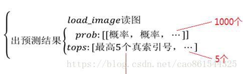
用vgg16实现图片识别

 vgg网络具体结构 

VGG源码包含的文件主要有app.py,vgg16.py,utils.py,Nclasses.py，vgg16.npy.

app.py:应用程序，实现图像识别

 

#coding:utf-8
import numpy as np
import tensorflow as tf
#引入绘图模块
import matplotlib.pyplot as plt
#引用自定义模块
import vgg16
import utils
from Nclasses import labels
 
testNum = input("input the number of test pictures:")
for i in range(testNum):
    img_path = raw_input('Input the path and image name:')
    #对待测试图像出预处理操作
    img_ready = utils.load_image(img_path) 
 
    #定义画图窗口，并指定窗口名称
    fig=plt.figure(u"Top-5 预测结果") 
 
    with tf.Session() as sess:
        #定义一个维度为[1, 224, 224, 3]的占位符
        images = tf.placeholder(tf.float32, [1, 224, 224, 3])
        #实例化出vgg
        vgg = vgg16.Vgg16() 
        #前向传播过程，调用成员函数，并传入待测试图像
        vgg.forward(images) 
        #将一个batch数据喂入网络，得到网络的预测输出
        probability = sess.run(vgg.prob, feed_dict={images:img_ready})
        #得到预测概率最大的五个索引值
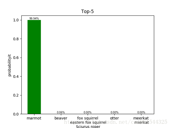
        top5 = np.argsort(probability[0])[-1:-6:-1]
        print "top5:",top5
        #定义两个list-对应概率值和实际标签
        values = []
        bar_label = []
        #枚举上面取出的五个索引值
        for n, i in enumerate(top5): 
            print "n:",n
            print "i:",i
            #将索引值对应的预测概率值取出并放入value
            values.append(probability[0][i]) 
            #将索引值对应的际标签取出并放入bar_label
            bar_label.append(labels[i]) 
            print i, ":", labels[i], "----", utils.percent(probability[0][i]) 
        
        #将画布分为一行一列，并把下图放入其中
        ax = fig.add_subplot(111) 
        #绘制柱状图
        ax.bar(range(len(values)), values, tick_label=bar_label, width=0.5, fc='g')
        #设置横轴标签
        ax.set_ylabel(u'probabilityit') 
        #添加标题
        ax.set_title(u'Top-5') 
        for a,b in zip(range(len(values)), values):
            #显示预测概率值
            ax.text(a, b+0.0005, utils.percent(b), ha='center', va = 'bottom', fontsize=7)   
        #显示图像
        plt.show() 

vgg16.py:读模型参数，搭建模型

#!/usr/bin/python
#coding:utf-8
 
import inspect
import os
import numpy as np
import tensorflow as tf
import time
import matplotlib.pyplot as plt
 
#样本RGB的平均值
VGG_MEAN = [103.939, 116.779, 123.68] 
 
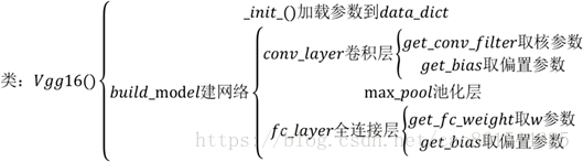
class Vgg16():
    def __init__(self, vgg16_path=None):
        if vgg16_path is None:
        #返回当前工作目录
            vgg16_path = os.path.join(os.getcwd(), "vgg16.npy") 
        #遍历其内键值对，导入模型参数
            self.data_dict = np.load(vgg16_path, encoding='latin1').item() 
 
    def forward(self, images):
        
        print("build model started")
    #获取前向传播开始时间
        start_time = time.time() 
    #逐个像素乘以255
        rgb_scaled = images * 255.0 
    #从GRB转换彩色通道到BRG
        red, green, blue = tf.split(rgb_scaled,3,3) 
    #减去每个通道的像素平均值，这种操作可以移除图像的平均亮度值
    #该方法常用在灰度图像上
        bgr = tf.concat([     
            blue - VGG_MEAN[0],
            green - VGG_MEAN[1],
            red - VGG_MEAN[2]],3)
        #构建VGG的16层网络（包含5段卷积，3层全连接），并逐层根据命名空间读取网络参数
    #第一段卷积，含有两个卷积层，后面接最大池化层，用来缩小图片尺寸
        self.conv1_1 = self.conv_layer(bgr, "conv1_1") 
    #传入命名空间的name，来获取该层的卷积核和偏置，并做卷积运算，最后返回经过激活函数后的值
        self.conv1_2 = self.conv_layer(self.conv1_1, "conv1_2")
    #根据传入的pooling名字对该层做相应的池化操作
        self.pool1 = self.max_pool_2x2(self.conv1_2, "pool1")
        
    #第二段卷积，包含两个卷积层，一个最大池化层
        self.conv2_1 = self.conv_layer(self.pool1, "conv2_1")
        self.conv2_2 = self.conv_layer(self.conv2_1, "conv2_2")
        self.pool2 = self.max_pool_2x2(self.conv2_2, "pool2")
 
        #第三段卷积，包含三个卷积层，一个最大池化层
        self.conv3_1 = self.conv_layer(self.pool2, "conv3_1")
        self.conv3_2 = self.conv_layer(self.conv3_1, "conv3_2")
        self.conv3_3 = self.conv_layer(self.conv3_2, "conv3_3")
        self.pool3 = self.max_pool_2x2(self.conv3_3, "pool3")
        
    #第四段卷积，包含三个卷积层，一个最大池化层
        self.conv4_1 = self.conv_layer(self.pool3, "conv4_1")
        self.conv4_2 = self.conv_layer(self.conv4_1, "conv4_2")
        self.conv4_3 = self.conv_layer(self.conv4_2, "conv4_3")
        self.pool4 = self.max_pool_2x2(self.conv4_3, "pool4")
        
    #第五段卷积，包含三个卷积层，一个最大池化层
        self.conv5_1 = self.conv_layer(self.pool4, "conv5_1")
        self.conv5_2 = self.conv_layer(self.conv5_1, "conv5_2")
        self.conv5_3 = self.conv_layer(self.conv5_2, "conv5_3")
        self.pool5 = self.max_pool_2x2(self.conv5_3, "pool5")
        
    #第六层全连接
    #根据命名空间name做加权求和运算
        self.fc6 = self.fc_layer(self.pool5, "fc6")
    #经过relu激活函数
        self.relu6 = tf.nn.relu(self.fc6) 
        
    #第七层全连接
        self.fc7 = self.fc_layer(self.relu6, "fc7")
        self.relu7 = tf.nn.relu(self.fc7)
        
    #第八层全连接
        self.fc8 = self.fc_layer(self.relu7, "fc8")
        self.prob = tf.nn.softmax(self.fc8, name="prob")
        
    #得到全向传播时间
        end_time = time.time() 
        print(("time consuming: %f" % (end_time-start_time)))
        
    #清空本次读取到的模型参数字典
        self.data_dict = None 
    
    #定义卷积运算    
    def conv_layer(self, x, name):
    #根据命名空间name找到对应卷积层的网络参数
        with tf.variable_scope(name): 
        #读到该层的卷积核
            w = self.get_conv_filter(name) 
        #卷积运算
            conv = tf.nn.conv2d(x, w, [1, 1, 1, 1], padding='SAME') 
            #读到偏置项
        conv_biases = self.get_bias(name) 
        #加上偏置，并做激活计算
            result = tf.nn.relu(tf.nn.bias_add(conv, conv_biases)) 
            return result
    
    #定义获取卷积核的参数
    def get_conv_filter(self, name):
    #根据命名空间从参数字典中获取对应的卷积核
        return tf.constant(self.data_dict[name][0], name="filter") 
    
    #定义获取偏置项的参数
    def get_bias(self, name):
    #根据命名空间从参数字典中获取对应的偏置项
        return tf.constant(self.data_dict[name][1], name="biases")
    
    #定义最大池化操作
    def max_pool_2x2(self, x, name):
        return tf.nn.max_pool(x, ksize=[1, 2, 2, 1], strides=[1, 2, 2, 1], padding='SAME', name=name)
    
    #定义全连接层的全向传播操作
    def fc_layer(self, x, name):
    #根据命名空间name做全连接层的计算
        with tf.variable_scope(name): 
        #获取该层的维度信息列表
            shape = x.get_shape().as_list() 
            dim = 1
            for i in shape[1:]:
        #将每层的维度相乘
                dim *= i 
        #改变特征图的形状，也就是将得到的多维特征做拉伸操作，只在进入第六层全连接层做该操作
            x = tf.reshape(x, [-1, dim])
        #读到权重值
            w = self.get_fc_weight(name) 
        #读到偏置项值
            b = self.get_bias(name) 
            #对该层输入做加权求和，再加上偏置
            result = tf.nn.bias_add(tf.matmul(x, w), b) 
            return result
    
    #定义获取权重的函数
    def get_fc_weight(self, name): 
    #根据命名空间name从参数字典中获取对应1的权重
        return tf.constant(self.data_dict[name][0], name="weights")

utils.py：读入图片，概率显示：

#!/usr/bin/python
#coding:utf-8
from skimage import io, transform
import numpy as np
import matplotlib.pyplot as plt
import tensorflow as tf
from pylab import mpl
 
mpl.rcParams['font.sans-serif']=['SimHei'] # 正常显示中文标签
mpl.rcParams['axes.unicode_minus']=False # 正常显示正负号
 
def load_image(path):
    fig = plt.figure("Centre and Resize")
    #传入读入图片的参数路径
    img = io.imread(path) 
    #将像素归一化处理到[0,1]
    img = img / 255.0 
    
    #将该画布分为一行三列，把下面的图像放在画布的第一个位置
    ax0 = fig.add_subplot(131)  
    #添加子标签
    ax0.set_xlabel(u'Original Picture') 
    #添加展示该图像
    ax0.imshow(img) 
    
    #找到该图像的最短边
    short_edge = min(img.shape[:2]) 
    #把图像的w和h分别减去最短边，并求平均
    y = (img.shape[0] - short_edge) / 2  
    x = (img.shape[1] - short_edge) / 2 
    #取出切分过的中心图像
    crop_img = img[y:y+short_edge, x:x+short_edge] 
    
    #把下面的图像放在画布的第二个位置
    ax1 = fig.add_subplot(132) 
    #添加子标签
    ax1.set_xlabel(u"Centre Picture") 
    #添加展示该图像
    ax1.imshow(crop_img)
    
    #resize成固定的imagesize
    re_img = transform.resize(crop_img, (224, 224)) 
    
    #把下面的图像放在画布的第三个位置
    ax2 = fig.add_subplot(133) 
    ax2.set_xlabel(u"Resize Picture") 
    ax2.imshow(re_img)
    #转换为需要的输入形状
    img_ready = re_img.reshape((1, 224, 224, 3))
 
    return img_ready
 
#定义百分比转换函数
def percent(value):
    return '%.2f%%' % (value * 100)

Nclasses.py：含lables字典，共1000个标签

vgg16.npy：网络参数，训练好的参数模型

app.py运行预测结果