【Tensorflow】实现简单的神经网络模型

在上一节我们简单说了一下简单的模型，有线性回归，Logistic模型以及KNN。

这次我们来说一下tensorflow的神经网络模型

无论是构建线性回归这种简单模型还是神经网络，步骤都是差不多的，inference,loss,training这大概的三个步骤。

下面这个例子仅仅是使用了激活函数，没有用到具体的神经网络

import tensorflow as tf
# 第一层的特征数
n_hidden1=256
# 第二层的特征数
n_hidden2=256
# 输入维度
n_input=784
# 输入占位符
x=tf.placeholder('float32',[None,n_input])
# 编码
def encoder(x):
    # 参数 tf,random_normal生成正太分布,第一个参数是shape
    weight1=tf.Variable(tf.random_normal([n_input,n_hidden1]))
    biases1=tf.Variable(tf.random_normal([n_hidden1]))
    weight2=tf.Variable(tf.random_normal([n_hidden1,n_hidden2]))
    biases2=tf.Variable(tf.random_normal([n_hidden2]))
    # 第一层,sigmoid是激活函数，神经元的非线性作用函数。输出范围是[0-1]，可以作为概率
    layer_1=tf.nn.sigmoid(tf.add(tf.matmul(x,weight1),biases1))
    # 第二层
    layer_2=tf.nn.sigmoid(tf.add(tf.matmul(x,weight2),biases2))
    return layer_2
# 解码
def decoder(x):
    # 参数
    weight1=tf.Variable(tf.random_normal([n_hidden2,n_hidden1]))
    biases1=tf.Variable(tf.random_normal([n_hidden1]))
    weight2=tf.Variable(tf.random_normal([n_hidden1,n_input]))
    biases2=tf.Variable(tf.random_normal([n_input]))
    #同理
    layer_1=tf.nn.sigmoid(tf.add(tf.matmul(x,weight1),biases1))
    layer_2=tf.nn.sigmoid(tf.add(tf.matmul(x,weight2),biases2))
    return layer_2
# 编码
encoder_op=encoder(x)
# 解码
decoder_op=decoder(encoder_op)
# 编码后解码的数据
y_pred=decoder_op
# 真实的数据
y_true=x
# 拟合模型时的参数
learning_rate=0.01
batch_size=50
training_epochs=1000
# 损失值
cost=tf.reduce_mean(tf.pow(y_true-y_pred,2))
# 优化器，RMSProp优化算法优化
optimizer=tf.train.RMSPropOptimizer(learning_rate).minimize(cost)
init=tf.global_variables_initializer()
with tf.Session() as sess:
    sess.run(init)
    # 分批训练
    total_batch=int(mnist.train.num_examples/batch_size)
    for  epoch in range(training_epochs):
        for i in range(total_batch):
            batch_xs,batch_ys=mnist.train.next_batch(batch_size)
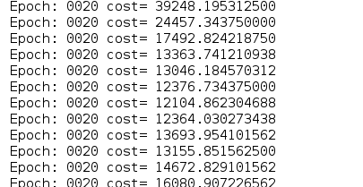
            _,c=sess.run([optimizer,cost],feed_dict={x:batch_xs})

除了上面注释所有的内容外，额外讲一下为什么要用sigmoid。sigmoid函数的形式是1/1+exp(e-x)。我们需要一个可以学习和表示

几乎任何东西的神经网络模型，以及可以将输入映射到输出的任意复杂函数。归于这一点，我们需要激活函数，使网络更加强大。如果不用激活函数的话，一个没有激活函数的神经网络不过是一个线性回归模型，功率有限，且误差非常大。如图就是没有用激活函数去训练的误差。还有就是tf.nn提供了神经网络的相关操作。

我们只要记住：“输入权值，添加偏移，激活函数”

另外关于RMSProp优化算法，这里有个转载他人的图片介绍。原文在此：点击打开链接

            

双向RNN的简单实现：

以下的代码是将MNIST图像数据集分割成序列，用LSTM模型记忆图像，然后根据图像预测类别 

import tensorflow as tf
# 这些参数应该是确定整个模型的数据shape之后才能确定的
n_steps=28
n_input=28
n_class=10
n_hidden=128
x=tf.placeholder('float',[None,n_steps,n_input])
y=tf.placeholder('float',[None,n_class])
weights={
    'out':tf.Variable(tf.random_normal([2*n_hidden,n_class]))
}
biases={
    'out':tf.Variable(tf.random_normal([n_class]))
}
def BiRNN(x,weights,biases):
    # transpose这个函数是转换tensor的维度,这行代码的意思是将第一维度和第二维度变换
    # 但是我不知道这行代码的意义是什么
    x=tf.transpose(x,[1,0,2])
    x=tf.reshape(x,[-1,n_input])
    # 将x分割成n_steps个[batch_size,n_input]tensor
    # 这个例子x就是28个[128,28]tensor
    # 但是我也不知道为什么要将数据转换为这样
    x=tf.split(x,n_steps,0)
    # 双向RNN
    lstm_fw_cell=rnn.BasicLSTMCell(n_hidden,forget_bias=1.0)
    lstm_bw_cell=rnn.BasicLSTMCell(n_hidden,forget_bias=1.0)
    outputs, _, _ = rnn.static_bidirectional_rnn(lstm_fw_cell, lstm_bw_cell, x, dtype=tf.float32)
    # 以线性激活返回预测值,用rnn inner loop的最后一个值
    # 从这里就可以确定参数的shape了
    # n_class是10,有两层神经网络,因此weights[2*n_hidden,n_class]
    return tf.matmul(outputs[-1],weights['out'])+biases['out']
# pred的shape是[?,10]
pred=BiRNN(x,weights,biases)
learning_rate=0.01
# softmax_cross_entropy_with_logits这个函数有两个参数logits,label
# 具体实现过程是首先对网络最后一层输出做一个softmax,然后softmax的输出向量做一个交叉熵
# 注意，这个函数的返回值是一个向量，如果要求loss，则要reduce_mean一下
cost=tf.reduce_mean(tf.nn.softmax_cross_entropy_with_logits(logits=pred,labels=y))
optimizer=tf.train.AdamOptimizer(learning_rate).minimize(cost)
correct_pred=tf.equal(tf.argmax(pred,1),tf.argmax(y,1))
accuracy=tf.reduce_mean(tf.cast(correct_pred,tf.float32))
init=tf.global_variables_initializer()
with tf.Session() as sess:
    sess.run(init)
    step=1
    batch_size=128
    training_iters=100000
    while step*batch_size<training_iters:
        batch_x,batch_y=mnist.train.next_batch(batch_size)
        # batch_x被转换为[128,28,28]格式的数据
        batch_x=batch_x.reshape((batch_size,n_steps,n_input))
        sess.run(optimizer,feed_dict={x:batch_x,y:batch_y})
        step+=1
    print('Done!')

在上面的代码中，我有几个问题没解决。第一就是为什么要对X进行transpose。第二就是双向RNN内部原理还没有弄懂。等到以后知道答案后我再来补。

卷积神经网络CNN：

从上述RNN的构建过程我们得知，如果要构建模型，我们需要知道怎么用模型去达成自己的目标，需要有个全局观念。

而这次CNN的构建，同样如此

learning_rate = 0.001
training_iters = 10000
batch_size = 120
display_step = 10
n_input = 784
n_classes = 10
dropout = 0.75
x = tf.placeholder(tf.float32, [None, n_input])
y = tf.placeholder(tf.float32, [None, n_classes])
keep_prob = tf.placeholder(tf.float32)


# strides指的是步长,即卷积核或者pooling窗口的滑动位移
def conv2d(x, W, bias, strides=1):
    # conv2d的几个参数是input,filter,strides,padding
    # input是指给定一个input的张量[batch,in_height,in_width,in_channels],batch个图像,大小为in_height*in_width,in_channels个通道
    # 过滤器filter[filter_height,filter_width,in_channels,out_channels],filter的大小是filter_height*filter_width,输入通道是in_channels,输出通道是out_channels4
    # 当padding为SAME时,输入和输出形状相同.
    x = tf.nn.conv2d(x, W, strides=[1, strides, strides, 1], padding='SAME')
    x = tf.nn.bias_add(x, bias)
    return tf.nn.relu(x)


# 池化使得特征具有平移不变性,从而得到更加鲁棒的特征
def maxpool2d(x, k=2):
    # max_pool有四个参数
    # 参数一vallue,池化层一般在卷积层后面
    # 参数二ksize,池化窗口的大小,一般是[1,height,width,1],不想在batch和channels上做池化,所以这两个维度设置为1
    # 参数三strides,步长
    # 参数四padding
    return tf.nn.max_pool(x, ksize=[1, k, k, 1], strides=[1, k, k, 1], padding='SAME')


# 构建CNN网络
def conv_net(x, weights, biases, dropout):
    x = tf.reshape(x, shape=[-1, 28, 28, 1])
    # 第一层卷积层
    conv1 = conv2d(x, weights['wc1'], biases['wc1'])
    # 池化层再将32个通道最大池化
    conv1 = maxpool2d(conv1, k=2)
    # 第二层卷积层
    conv2 = conv2d(conv1, weights['wc2'], biases['wc2'])
    # 池化层
    conv2 = maxpool2d(conv2, k=2)
    # 全连接层
    # 卷积层的输出结果形式是[?,7,7,64] ,7的得来是28/(2*2)
    # 将卷积层的结果转化为[-1,7*7*64]的形式
    fc1 = tf.reshape(conv2, [-1, weights['wd1'].get_shape().as_list()[0]])
    fc1 = tf.add(tf.matmul(fc1, weights['wd1']), biases['wd1'])
    # 用relu激活函数
    fc1 = tf.nn.relu(fc1)
    # 输出的数据被剔除了1/dropout
    fc1 = tf.nn.dropout(fc1, dropout)
    # 返回的是被剔除后的线性激活
    out = tf.add(tf.matmul(fc1, weights['out']), biases['out'])
    return out



weights = {
    # 这个第一层卷积层的参数表示filter的大小是5*5,输入通道是1,输出通道是32
    'wc1': tf.Variable(tf.random_normal([5, 5, 1, 32])),
    # 5*5图像,32个输入通道,64个输出通道
    'wc2': tf.Variable(tf.random_normal([5, 5, 32, 64])),
    # 因为conv2的输出shape是[?,7,7,64],所以参数的形式就定了
    'wd1': tf.Variable(tf.random_normal([7 * 7 * 64, 1024])),
    'out': tf.Variable(tf.random_normal([1024, n_classes]))
}
biases = {
    'wc1': tf.Variable(tf.random_normal([32])),
    'wc2': tf.Variable(tf.random_normal([64])),
    'wd1': tf.Variable(tf.random_normal([1024])),
    'out': tf.Variable(tf.random_normal([n_classes]))
}

pred = conv_net(x, weights, biases, keep_prob)
cost = tf.reduce_mean(tf.nn.softmax_cross_entropy_with_logits(logits=pred, labels=y))
optimizer = tf.train.AdamOptimizer(learning_rate).minimize(cost)
init=tf.global_variables_initializer()
with tf.Session() as sess:
    step=1
    sess.run(init)
    while batch_size*step<training_iters:
        # batch_x是[?,784]形状的
        batch_x,batch_y=mnist.train.next_batch(batch_size)
        sess.run(optimizer,feed_dict={x:batch_x,y:batch_y,keep_prob:dropout})
        step+=1
print('Done!')

在构建上述模型中，我感觉到参数和输入输出的shape要定下来是非常重要的.除此之外，上述代码只是去拟合了模型，如果我们想要知道模型的好坏，则需要以下代码.

correct_pred=tf.equal(tf.argmax(pred,1),tf.argmax(y,1))
accuracy=tf.reduce_mean(tf.cast(correct_pred,tf.float32))

accuracy就是预测的准确率