学习目标:在 TensorFlow 中使用 LinearRegressor 类并基于单个输入特征预测各城市街区的房屋价值中位数,使用均方根误差 (RMSE) 评估模型预测的准确率,通过调整模型的超参数提高模型准确率。
import math
from IPython import display    # display模块可以决定显示的内容以何种格式显示
from matplotlib import cm    # matplotlib为python的2D绘图库# cm为颜色映射表
from matplotlib import gridspec    # 使用 GridSpec 自定义子图位置
from matplotlib import pyplot as plt    # pyplot提供了和matlab类似的绘图API,方便用户快速绘制2D图表
import numpy as np    # numpy为python的科学计算包,提供了许多高级的数值编程工具
import pandas as pd    # pandas是基于numpy的数据分析包,是为了解决数据分析任务而创建的
from sklearn import metrics    # sklearn(scikit-_learn_)是一个机器学习算法库,包含了许多种机器学习得方式
# * Classification 分类# * Regression 回归
# * Clustering 非监督分类# * Dimensionality reduction 数据降维
# * Model Selection 模型选择# * Preprocessing 数据预处理
# metrics:度量(字面意思),它提供了很多模块可以为第三方库或者应用提供辅助统计信息
import tensorflow as tf    # tensorflow是谷歌的机器学习框架
from tensorflow.python.data import Dataset    # Dataset无比强大得数据集

tf.logging.set_verbosity(tf.logging.ERROR)
pd.options.display.max_rows = 10    # 为了观察数据方便,最多只显示10行数据
pd.options.display.float_format = '{:.1f}'.format

california_housing_dataframe = pd.read_csv("https://storage.googleapis.com/mledu-datasets/california_housing_train.csv", sep=",")
 #加载数据集

california_housing_dataframe = california_housing_dataframe.reindex(
    np.random.permutation(california_housing_dataframe.index))
california_housing_dataframe["median_house_value"] /= 1000.0
california_housing_dataframe    #对数据进行预处理将median_house_value调整为以千为单位。

california_housing_dataframe.describe() #检查数据my_feature = california_housing_dataframe[["total_rooms"]]# Define the input feature: total_rooms.
# 取数据集中得'total_rooms'这一列作为输入特征
# Configure a numeric feature column for total_rooms.
# 将一个名叫"total_rooms"的特征列定义为**数值数据** ,这样的定义结果存在feature_columns中
# 即上文所说得**特征列**中,这时候特征列其实只是一个存储了分类信息的集合,具体使用的时候需要# 特征集合和特征列结合起来,分类器才能识别的呢
feature_columns = [tf.feature_column.numeric_column("total_rooms")]# Define the label.# 将"median_house_value"列的数据从数据集中取出作为target,定义我们学习的目标
targets = california_housing_dataframe["median_house_value"]# Use gradient descent as the optimizer for training the model.
my_optimizer=tf.train.GradientDescentOptimizer(learning_rate=0.0000001)
my_optimizer = tf.contrib.estimator.clip_gradients_by_norm(my_optimizer, 5.0)
# 这里的clip_by_norm是指对梯度进行裁剪,通过控制梯度的最大范式,防止梯度爆炸的问题,是一种
# 比较常用的梯度规约的方式。
linear_regressor = tf.estimator.LinearRegressor(
feature_columns=feature_columns,
optimizer=my_optimizer
)
# Configure the linear regression model with our feature columns and optimizer
# Set a learning rate of 0.0000001 for Gradient Descent.# 线性回归模型,tf.estimator.LinearRegressor是tf.estimator.Estimator的子类
# 传入参数为**特征**列和刚才配置的**优化器**,至此线性回归模型就配置的差不多啦
# 前期需要配置模型,所以是与具体数据(特征值,目标值是无关的)def my_input_fn(features, targets, batch_size=1, shuffle=True, num_epochs=None):
# 自定义个输入函数
# 输入的参数分别为
# features:特征值(房间数量)
# targets: 目标值(房屋价格中位数)
# batch_size:每次处理训练的样本数(这里设置为1)
# shuffle: 如果 `shuffle` 设置为 `True`,则我们会对数据进行随机处理
# num_epochs:将默认值 `num_epochs=None` 传递到 `repeat()`,输入数据会无限期重复
features = {key:np.array(value) for key,value in dict(features).items()}
# dict(features).items():将输入的特征值转换为dictinary(python的一种数据类型,
# 通过for语句遍历,得到其所有的一一对应的值(key:value)
ds = Dataset.from_tensor_slices((features,targets)) # warning: 2GB limit
# Dataset.from_tensor_slices((features,targets))将输入的两个参数拼接组合起来,
# 形成一组一组的**切片**张量{(房间数,价格),(房间数,价格)....}
ds = ds.batch(batch_size).repeat(num_epochs)
# batch(batch_size):将ds数据集按照batch_size大小组合成一个batch
# repeat(num_epochs):repeat代表从ds这个数据集要重复读取几次,在这里num_epochs=None
# 代表无限次重复下去,但是因为ds数据集有容量上限,所以会在上限出停止重复
if shuffle:
ds = ds.shuffle(buffer_size=10000)
# Shuffle the data, if specified
# 现在ds中得数据集已经时按照batchsize组合成得一个一个batch,存放在队列中,并且是重复了n次
# 这样子得话,不断重复,后面数据是没有意义,所以要将其随机打乱
# shuffle(buffer_size=10000):表示打乱得时候使用得buffer大小是10000,即ds中按顺序取10000个出来
# 打乱放回去,接着从后面再取10000个,按顺序来
features, labels = ds.make_one_shot_iterator().get_next()
# Return the next batch of data
# make_one_shot_iterator():最简单的一种迭代器,仅会对数据集遍历一遍
# make_one_shot_iterator().get_next():迭代的时候返回所有的结果
return features, labels
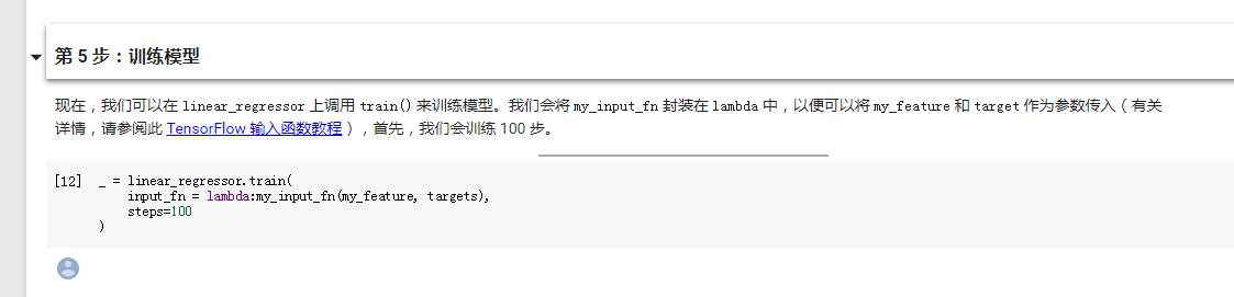
# 向 LinearRegressor 返回下一批数据_ = linear_regressor.train(
input_fn = lambda:my_input_fn(my_feature, targets),
steps=100
)第6步:评估模型
# 上一步已经将数据输入,并训练了一百步,所以现在的模型的参数是已经调整过的
# 现在我们来获得**误差**,对误差进行分析,以衡量训练了一百步的模型效果怎么样
# 获取误差的方式很简单,还是采用原来的数据集输入,这次不是训练,而是直接预测,返回预测结果
prediction_input_fn =lambda: my_input_fn(my_feature, targets, num_epochs=1, shuffle=False)
predictions = linear_regressor.predict(input_fn=prediction_input_fn)
predictions = np.array([item['predictions'][0] for item in predictions])
# 将预测结果取出,格式化为numpy数组,来进行误差分析
mean_squared_error = metrics.mean_squared_error(predictions, targets)
# 计算均方误差(MSE),即Sum((target-predictions)²)/N,
root_mean_squared_error = math.sqrt(mean_squared_error)
# 再对均方误差开根,得到均方根误差(RMSE),目的就是看看预测值和真实的target相差了多少
print "Mean Squared Error (on training data): %0.3f" % mean_squared_error
print "Root Mean Squared Error (on training data): %0.3f" % root_mean_squared_error
# 输出MSE和RMSEMean Squared Error (on training data): 56367.025
Root Mean Squared Error (on training data): 237.417min_house_value = california_housing_dataframe["median_house_value"].min()
max_house_value = california_housing_dataframe["median_house_value"].max()
min_max_difference = max_house_value - min_house_value
print "Min. Median House Value: %0.3f" % min_house_value
print "Max. Median House Value: %0.3f" % max_house_value
print "Difference between Min. and Max.: %0.3f" % min_max_difference
print "Root Mean Squared Error: %0.3f" % root_mean_squared_error
输出结果是:
Min. Median House Value: 14.999
Max. Median House Value: 500.001
Difference between Min. and Max.: 485.002
Root Mean Squared Error: 237.417calibration_data = pd.DataFrame()
# 使用pdndas的工具来对数据简单处理分析
calibration_data["predictions"] = pd.Series(predictions)
calibration_data["targets"] = pd.Series(targets)
calibration_data.describe()
# pd.Series就是将参数中的list(一维的矩阵),添加到其中,具体效果看输出的表格sample = california_housing_dataframe.sample(n=300)
# Get the min and max total_rooms values.
x_0 = sample["total_rooms"].min()
x_1 = sample["total_rooms"].max()
weight = linear_regressor.get_variable_value('linear/linear_model/total_rooms/weights')[0]
bias = linear_regressor.get_variable_value('linear/linear_model/bias_weights')
# 从目前的训练模型中取出训练得到的weight(权重)和bias(b:y=w1x1+w2x2+...+b其中的b)
y_0 = weight * x_0 + bias
y_1 = weight * x_1 + bias
# 使用目前训练得到权值去预测出x_0和x_1对应的y_0和y_1(这样可以得到预测的两个点的坐标,因为训练得到的预测结果是线性的,只要知道直线端点就ok)
plt.plot([x_0, x_1], [y_0, y_1], c='r')
# 还记得一开始导入的一个2D图形库matplotlib吗,其是python的最主要的可视化库
# 可以利用其绘制散点图、直方图和箱形图,及修改图表属性等
# 下面使用其plot(二维线条画图函数),用两个点画线,c='r'是线条参数,红色
plt.ylabel("median_house_value")
plt.xlabel("total_rooms")
# 设置坐标轴lable
plt.scatter(sample["total_rooms"], sample["median_house_value"])
# scatter()绘制散点图,在此绘制sample中的对应的total_rooms和median_house_value的散点图
plt.show()
模型调整第2步:调整模型超参数
# 定义个函数融合上面所有的操作,以下是参数说明,并顺便复习以下上面的内容
# learning_rate:学习速率(步长),可以调节梯度下降的速度
# steps:训练步数,越久效果一般会越准确,但花费的时间也是越多的
# batch_size:每次处理训练的样本数(将原来数据打包成一块一块的,块的大小)
# input_feature:输入的特征
def train_model(learning_rate, steps, batch_size, input_feature="total_rooms"):
periods = 10
# 将步长分十份,用于每训练十分之一的步长就输出一次结果
steps_per_period = steps / periods
# 以下是准备数据,分别是my_feature_data 和 targets
my_feature = input_feature
my_feature_data = california_housing_dataframe[[my_feature]]
my_label = "median_house_value"
targets = california_housing_dataframe[my_label]
# 创建特征列
feature_columns = [tf.feature_column.numeric_column(my_feature)]
# 创建输入函数(训练和预测)
training_input_fn = lambda:my_input_fn(my_feature_data, targets, batch_size=batch_size)
prediction_input_fn = lambda: my_input_fn(my_feature_data, targets, num_epochs=1, shuffle=False)
# 创建线性回归模型
my_optimizer = tf.train.GradientDescentOptimizer(learning_rate=learning_rate)
my_optimizer = tf.contrib.estimator.clip_gradients_by_norm(my_optimizer, 5.0)
linear_regressor = tf.estimator.LinearRegressor(
feature_columns=feature_columns,
optimizer=my_optimizer
)
# 设置每个阶段的输出
# 新建绘画窗口,自定义画布的大小为15*6
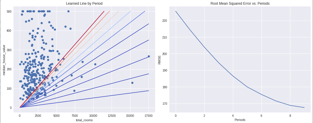
plt.figure(figsize=(15, 6))
# 设置画布划分以及图像在画布上输出的位置1行2列,绘制在第1个位置
plt.subplot(1, 2, 1)
plt.title("Learned Line by Period")
plt.ylabel(my_label)
plt.xlabel(my_feature)
sample = california_housing_dataframe.sample(n=300)
plt.scatter(sample[my_feature], sample[my_label])
# np.linspace(-1, 1, periods):用于输出等差数列,起始-1,结尾1,periods=10,10等分(不写的话默认50等分)
# cm.coolwarm(x):设置颜色,用于十条线显示不同颜色
colors = [cm.coolwarm(x) for x in np.linspace(-1, 1, periods)]
# 周期评估并输出(把训练分十次,并输出)
print "Training model..."
print "RMSE (on training data):"
root_mean_squared_errors = []
for period in range (0, periods):
linear_regressor.train(
input_fn=training_input_fn,
steps=steps_per_period
)
predictions = linear_regressor.predict(input_fn=prediction_input_fn)
predictions = np.array([item['predictions'][0] for item in predictions])
root_mean_squared_error = math.sqrt(
metrics.mean_squared_error(predictions, targets))
print " period %02d : %0.2f" % (period, root_mean_squared_error)
root_mean_squared_errors.append(root_mean_squared_error)
# 取出十次训练得到的w和b,用于绘制
y_extents = np.array([0, sample[my_label].max()])
weight = linear_regressor.get_variable_value('linear/linear_model/%s/weights' % input_feature)[0]
bias = linear_regressor.get_variable_value('linear/linear_model/bias_weights')
x_extents = (y_extents - bias) / weight
x_extents = np.maximum(np.minimum(x_extents,
sample[my_feature].max()),
sample[my_feature].min())
y_extents = weight * x_extents + bias
plt.plot(x_extents, y_extents, color=colors[period])
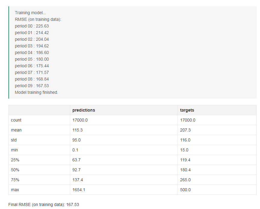
print "Model training finished."
# 输出RMSE曲线图
plt.subplot(1, 2, 2)
plt.ylabel('RMSE')
plt.xlabel('Periods')
plt.title("Root Mean Squared Error vs. Periods")
plt.tight_layout()
plt.plot(root_mean_squared_errors)
# 输出预测target的对比
calibration_data = pd.DataFrame()
calibration_data["predictions"] = pd.Series(predictions)
calibration_data["targets"] = pd.Series(targets)
display.display(calibration_data.describe())
print "Final RMSE (on training data): %0.2f" % root_mean_squared_error# 调用train_model
# learning_rate=0.00002:学习速率翻倍,有限步长可能会计算的更接近
# steps=500:训练500步
# batch_size=5:一批5组数据
train_model(
learning_rate=0.00002,
steps=500,
batch_size=5
)
学习过程中的疑问点总结
疑问点一:在定义输入函数的时候,这一行是什么意思?
features = {key:np.array(value) for key,value in dict(features).items()答:这里有两个问题点,一个是字典类型的数据,一个是items()函数的用法。
字典是一种变量数据的格式,特点在于“键-值“对应,可以通过键找到对应的值,就行找到门牌号就可以找房子的东西一样,这里的门牌号(键)是必须唯一的,即不能和其他门牌号(键)重复,所以一般为数字或字符串。而房子里的内容可以试任意的,可以有多种格式,也可重复,就像1号房子里有蛋糕,2号房子里也可以有一个一模一样的蛋糕。
字典详细的使用方法可参考:http://www.runoob.com/python/python-dictionary.html
字典的解释说明可参考:https://zhuanlan.zhihu.com/p/29034557
items()是一个遍历函数,大概的意思就是把键和值一一对应起来,也就是把门牌号排好(不一定按顺序),然后把各种东西放到各自的房子里面。
items()函数的具体用法参考:http://www.runoob.com/python/att-dictionary-items.html
疑问点二:这两行指令有什么作用,或者说两行指令实现的混洗数据的效果时什么样子,有什么意义。
    # Shuffle the data, if specified
    if shuffle:
      ds = ds.shuffle(buffer_size=10000)
答:这个根据注释里面的解释已经比较清楚了
疑问点三:这一行指令有什么作用?
ds.make_one_shot_iterator().get_next()答:注释说明为:
关于迭代器的具体解释参考:https://www.cnblogs.com/huxi/archive/2011/07/01/2095931.html
疑问点四:
说明中提到“我们会将 my_input_fn 封装在 lambda 中”lamda是什么,有什么作用?
答:lambda是一种匿名表达式,我们经常会遇到一种情况,某一个表达式可能只需要使用一次,还需要对这个表达式进行定义和命名,而使用lambda就可以解决这个问题,让程式书写更加简洁。
关于lambda 的解释参考:https://www.zhihu.com/question/20125256
疑问点五:这行指令是什么意思?
# Format predictions as a NumPy array, so we can calculate error metrics.
predictions = np.array([item['predictions'][0] for item in predictions])
答:这条指令的意思是将预测结果取出,格式化为numpy数组,以便进行误差分析。
本文请结合Google 机器学习,编程练习:使用TensorFlow的起始步骤一起观看
编程练习地址:https://colab.research.google.com/notebooks/mlcc/first_steps_with_tensor_flow.ipynb?hl=zh-cn
注释部分多引用于:https://segmentfault.com/a/1190000013807691