tensorflow 波士顿房价预测LSTM/RNN tensorboard 完整代码

在tensorflow里RNN才是做回归计算的正规军，其中LSTM更是让人工智能有了记忆，如果cnn最适合做的是图像识别，那么LSTM就是视频识别。网上的教程多是用正余弦数据在做预测，输入输出都是一维，我这用波士顿房价，输入是13个特征！

注意与前面两个模型不同的是，没有用train_test_split把训练数据分割，而是用的时序数据。

代码中注释比较少，不明白的可以看周莫烦的视频！

https://morvanzhou.github.io/tutorials/machine-learning/tensorflow/5-09-RNN3/

# 参考https://morvanzhou.github.io/tutorials/machine-learning/tensorflow/5-09-RNN3/
from sklearn.datasets import load_boston

from sklearn import preprocessing
import tensorflow as tf
import numpy as np

# 波士顿房价数据
boston = load_boston()
x = boston.data
y = boston.target

print( '波士顿数据X:',x.shape) # (506, 13)
# print(x[::100])
print( '波士顿房价Y:',y.shape)
# print(y[::100])
# 数据标准化
ss_x = preprocessing.StandardScaler()
train_x = ss_x.fit_transform(x)
ss_y = preprocessing.StandardScaler()
train_y = ss_y.fit_transform(y.reshape( -1, 1))

BATCH_START = 0 # 建立 batch data 时候的 index
TIME_STEPS = 10 # backpropagation through time 的 time_steps
BATCH_SIZE = 30
INPUT_SIZE = 13 # sin 数据输入 size
OUTPUT_SIZE = 1 # cos 数据输出 size
CELL_SIZE = 10 # RNN 的 hidden unit size
LR = 0.006 # learning rate

def get_batch_boston():
global train_x, train_y,BATCH_START, TIME_STEPS
x_part1 = train_x[BATCH_START : BATCH_START+TIME_STEPS*BATCH_SIZE]
y_part1 = train_y[BATCH_START : BATCH_START+TIME_STEPS*BATCH_SIZE]
print( '时间段=', BATCH_START, BATCH_START + TIME_STEPS * BATCH_SIZE)


seq =x_part1.reshape((BATCH_SIZE, TIME_STEPS ,INPUT_SIZE))
res =y_part1.reshape((BATCH_SIZE, TIME_STEPS , 1))

BATCH_START += TIME_STEPS

# returned seq, res and xs: shape (batch, step, input)
#np.newaxis 用来增加一个维度 变为三个维度，第三个维度将用来存上一批样本的状态
return [seq , res ]


def get_batch():
global BATCH_START, TIME_STEPS
# xs shape (50batch, 20steps)
xs = np.arange(BATCH_START, BATCH_START+TIME_STEPS*BATCH_SIZE).reshape((BATCH_SIZE, TIME_STEPS)) / ( 10*np.pi)
print( 'xs.shape=',xs.shape)
seq = np.sin(xs)
res = np.cos(xs)
BATCH_START += TIME_STEPS
# import matplotlib.pyplot as plt
# plt.plot(xs[0, :], res[0, :], 'r', xs[0, :], seq[0, :], 'b--')
# plt.show()
print( '增加维度前:',seq.shape)
print( seq[: 2])
print( '增加维度后:',seq[:, :, np.newaxis].shape)
print(seq[: 2])
# returned seq, res and xs: shape (batch, step, input)
#np.newaxis 用来增加一个维度 变为三个维度，第三个维度将用来存上一批样本的状态
return [seq[:, :, np.newaxis], res[:, :, np.newaxis], xs]


class LSTMRNN(object):
def __init__(self, n_steps, input_size, output_size, cell_size, batch_size):
'''
:param n_steps: 每批数据总包含多少时间刻度
:param input_size: 输入数据的维度
:param output_size: 输出数据的维度 如果是类似价格曲线的话，应该为1
:param cell_size: cell的大小
:param batch_size: 每批次训练数据的数量
'''
self.n_steps = n_steps
self.input_size = input_size
self.output_size = output_size
self.cell_size = cell_size
self.batch_size = batch_size
with tf.name_scope( 'inputs'):
self.xs = tf.placeholder(tf.float32, [ None, n_steps, input_size], name= 'xs') #xs 有三个维度
self.ys = tf.placeholder(tf.float32, [ None, n_steps, output_size], name= 'ys') #ys 有三个维度
with tf.variable_scope( 'in_hidden'):
self.add_input_layer()
with tf.variable_scope( 'LSTM_cell'):
self.add_cell()
with tf.variable_scope( 'out_hidden'):
self.add_output_layer()
with tf.name_scope( 'cost'):
self.compute_cost()
with tf.name_scope( 'train'):
self.train_op = tf.train.AdamOptimizer(LR).minimize(self.cost)
#增加一个输入层
def add_input_layer(self,):
# l_in_x:(batch*n_step, in_size),相当于把这个批次的样本串到一个长度1000的时间线上，每批次50个样本，每个样本20个时刻
l_in_x = tf.reshape(self.xs, [ -1, self.input_size], name= '2_2D') #-1 表示任意行数
# Ws (in_size, cell_size)
Ws_in = self._weight_variable([self.input_size, self.cell_size])
# bs (cell_size, )
bs_in = self._bias_variable([self.cell_size,])
# l_in_y = (batch * n_steps, cell_size)
with tf.name_scope( 'Wx_plus_b'):
l_in_y = tf.matmul(l_in_x, Ws_in) + bs_in
# reshape l_in_y ==> (batch, n_steps, cell_size)
self.l_in_y = tf.reshape(l_in_y, [ -1, self.n_steps, self.cell_size], name= '2_3D')

#多时刻的状态叠加层
def add_cell(self):
lstm_cell = tf.nn.rnn_cell.BasicLSTMCell(self.cell_size, forget_bias= 1.0, state_is_tuple= True)
with tf.name_scope( 'initial_state'):
self.cell_init_state = lstm_cell.zero_state(self.batch_size, dtype=tf.float32)
#time_major=False 表示时间主线不是第一列batch
self.cell_outputs, self.cell_final_state = tf.nn.dynamic_rnn(
lstm_cell, self.l_in_y, initial_state=self.cell_init_state, time_major= False)

# 增加一个输出层
def add_output_layer(self):
# shape = (batch * steps, cell_size)
l_out_x = tf.reshape(self.cell_outputs, [ -1, self.cell_size], name= '2_2D')
Ws_out = self._weight_variable([self.cell_size, self.output_size])
bs_out = self._bias_variable([self.output_size, ])
# shape = (batch * steps, output_size)
with tf.name_scope( 'Wx_plus_b'):
self.pred = tf.matmul(l_out_x, Ws_out) + bs_out #预测结果

def compute_cost(self):
losses = tf.nn.seq2seq.sequence_loss_by_example(
[tf.reshape(self.pred, [ -1], name= 'reshape_pred')],
[tf.reshape(self.ys, [ -1], name= 'reshape_target')],
[tf.ones([self.batch_size * self.n_steps], dtype=tf.float32)],
average_across_timesteps= True,
softmax_loss_function=self.ms_error,
name= 'losses'
)
with tf.name_scope( 'average_cost'):
self.cost = tf.div(
tf.reduce_sum(losses, name= 'losses_sum'),
self.batch_size,
name= 'average_cost')
tf.scalar_summary( 'cost', self.cost)

def ms_error(self, y_pre, y_target):
return tf.square(tf.sub(y_pre, y_target))

def _weight_variable(self, shape, name='weights'):
initializer = tf.random_normal_initializer(mean= 0., stddev= 1.,)
return tf.get_variable(shape=shape, initializer=initializer, name=name)

def _bias_variable(self, shape, name='biases'):
initializer = tf.constant_initializer( 0.1)
return tf.get_variable(name=name, shape=shape, initializer=initializer)


if __name__ == '__main__':
seq, res = get_batch_boston()

model = LSTMRNN(TIME_STEPS, INPUT_SIZE, OUTPUT_SIZE, CELL_SIZE, BATCH_SIZE)
sess = tf.Session()
merged = tf.merge_all_summaries()
writer = tf.train.SummaryWriter( "logs", sess.graph)
# tf.initialize_all_variables() no long valid from
# 2017-03-02 if using tensorflow >= 0.12
sess.run(tf.global_variables_initializer())
# relocate to the local dir and run this line to view it on Chrome (http://0.0.0.0:6006/):
# $ tensorboard --logdir='logs'
for j in range( 200): #训练200次
pred_res= None
for i in range( 20): #把整个数据分为20个时间段
seq, res = get_batch_boston()

if i == 0:
feed_dict = {
model.xs: seq,
model.ys: res,
# create initial state
}
else:
feed_dict = {
model.xs: seq,
model.ys: res,
model.cell_init_state: state # use last state as the initial state for this run
}

_, cost, state, pred = sess.run(
[model.train_op, model.cost, model.cell_final_state, model.pred],
feed_dict=feed_dict)
pred_res=pred


result = sess.run(merged, feed_dict)
writer.add_summary(result, i)
print( '{0} cost: '.format(j ), round(cost, 4))
BATCH_START= 0 #从头再来一遍

# 画图
print( "结果:",pred_res.shape)
#与最后一次训练所用的数据保持一致
train_y = train_y[ 190: 490]
print( '实际',train_y.flatten().shape)

r_size=BATCH_SIZE * TIME_STEPS
###画图###########################################################################
import matplotlib.pyplot as plt
fig = plt.figure(figsize=( 20, 3)) # dpi参数指定绘图对象的分辨率，即每英寸多少个像素，缺省值为80
axes = fig.add_subplot( 1, 1, 1)
#为了方便看，只显示了后100行数据
line1,=axes.plot(range( 100), pred.flatten()[ -100:] , 'b--',label= 'rnn计算结果')
#line2,=axes.plot(range(len(gbr_pridict)), gbr_pridict, 'r--',label='优选参数')
line3,=axes.plot(range( 100), train_y.flatten()[ - 100:], 'r',label= '实际')

axes.grid()
fig.tight_layout()
#plt.legend(handles=[line1, line2,line3])
plt.legend(handles=[line1, line3])
plt.title( '递归神经网络')
plt.show()

本文原址：http://blog.csdn.net/baixiaozhe/article/details/54410313
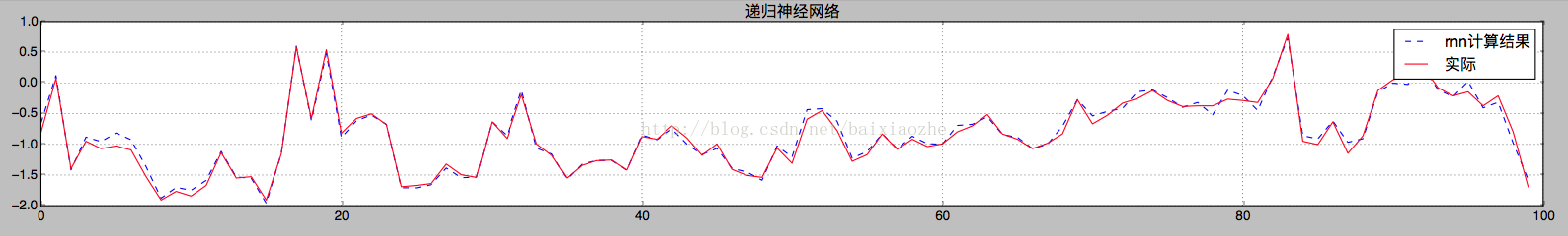
lstm输入和输出都是时序数据，是尊重时间的，和上两篇用的交叉数据集是不一样的，所以 结果是这样的：