三十分钟理解：线性插值，双线性插值Bilinear Interpolation算法

线性插值

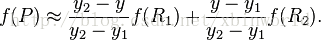
先讲一下线性插值：已知数据 (x0, y0) 与 (x1, y1)，要计算 [x0, x1] 区间内某一位置 x 在直线上的y值（反过来也是一样，略）：

y - y 0 x - x 0 = y 1 - y 0 x 1 - x 0

$\begin{equation} \frac{y - y_0}{x - x_0} = \frac{y_1 - y_0}{x_1 - x_0} \end{equation}$

y = x 1 - x x 1 - x 0 y 0 + x - x 0 x 1 - x 0 y 1

$\begin{equation} y = \frac{x_1 - x}{x_1 - x_0}y_0 +\frac{x - x_0}{x_1 - x_0}y_1 \end{equation}$

上面比较好理解吧，仔细看就是用x和x0，x1的距离作为一个权重，用于y0和y1的加权。双线性插值本质上就是在两个方向上做线性插值。

双线性插值

在数学上，双线性插值是有两个变量的插值函数的线性插值扩展，其核心思想是在两个方向分别进行一次线性插值[1]。见下图：

这里写图片描述

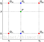
假如我们想得到未知函数 f 在点 P = (x, y) 的值，假设我们已知函数 f 在 Q11 = (x1, y1)、Q12 = (x1, y2), Q21 = (x2, y1) 以及 Q22 = (x2, y2) 四个点的值。最常见的情况，f就是一个像素点的像素值。首先在 x 方向进行线性插值，得到

这里写图片描述

然后在 y 方向进行线性插值，得到

这里写图片描述

综合起来就是双线性插值最后的结果：

这里写图片描述

由于图像双线性插值只会用相邻的4个点，因此上述公式的分母都是1。opencv中的源码如下，用了一些优化手段，比如用整数计算代替float（下面代码中的*2048就是变11位小数为整数，最后有两个连乘，因此>>22位），以及源图像和目标图像几何中心的对齐
SrcX=(dstX+0.5)* (srcWidth/dstWidth) -0.5
SrcY=(dstY+0.5) * (srcHeight/dstHeight)-0.5，

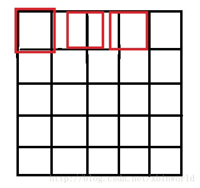
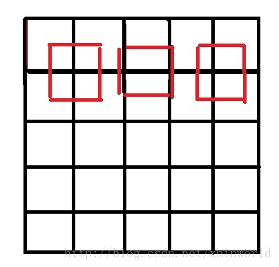
这个要重点说一下，源图像和目标图像的原点（0，0）均选择左上角，然后根据插值公式计算目标图像每点像素，假设你需要将一幅5x5的图像缩小成3x3，那么源图像和目标图像各个像素之间的对应关系如下。如果没有这个中心对齐，根据基本公式去算，就会得到左边这样的结果；而用了对齐，就会得到右边的结果：

这里写图片描述

cv::Mat matSrc, matDst1, matDst2;  

matSrc = cv::imread("lena.jpg", 2 | 4);  
matDst1 = cv::Mat(cv::Size(800, 1000), matSrc.type(), cv::Scalar::all(0));  
matDst2 = cv::Mat(matDst1.size(), matSrc.type(), cv::Scalar::all(0));  

double scale_x = (double)matSrc.cols / matDst1.cols;  
double scale_y = (double)matSrc.rows / matDst1.rows;  

uchar* dataDst = matDst1.data;  
int stepDst = matDst1.step;  
uchar* dataSrc = matSrc.data;  
int stepSrc = matSrc.step;  
int iWidthSrc = matSrc.cols;  
int iHiehgtSrc = matSrc.rows;  

for (int j = 0; j < matDst1.rows; ++j)  
{  
    float fy = (float)((j + 0.5) * scale_y - 0.5);  
    int sy = cvFloor(fy);  
    fy -= sy;  
    sy = std::min(sy, iHiehgtSrc - 2);  
    sy = std::max(0, sy);  

    short cbufy[2];  
    cbufy[0] = cv::saturate_cast<short>((1.f - fy) * 2048);  
    cbufy[1] = 2048 - cbufy[0];  

    for (int i = 0; i < matDst1.cols; ++i)  
    {  
        float fx = (float)((i + 0.5) * scale_x - 0.5);  
        int sx = cvFloor(fx);  
        fx -= sx;  

        if (sx < 0) {  
            fx = 0, sx = 0;  
        }  
        if (sx >= iWidthSrc - 1) {  
            fx = 0, sx = iWidthSrc - 2;  
        }  

        short cbufx[2];  
        cbufx[0] = cv::saturate_cast<short>((1.f - fx) * 2048);  
        cbufx[1] = 2048 - cbufx[0];  

        for (int k = 0; k < matSrc.channels(); ++k)  
        {  
            *(dataDst+ j*stepDst + 3*i + k) = (*(dataSrc + sy*stepSrc + 3*sx + k) * cbufx[0] * cbufy[0] +   
                *(dataSrc + (sy+1)*stepSrc + 3*sx + k) * cbufx[0] * cbufy[1] +   
                *(dataSrc + sy*stepSrc + 3*(sx+1) + k) * cbufx[1] * cbufy[0] +   
                *(dataSrc + (sy+1)*stepSrc + 3*(sx+1) + k) * cbufx[1] * cbufy[1]) >> 22;  
        }  
    }  
}  
cv::imwrite("linear_1.jpg", matDst1);  

cv::resize(matSrc, matDst2, matDst1.size(), 0, 0, 1);  
cv::imwrite("linear_2.jpg", matDst2);

好了，本篇到这里，欢迎大家分享转载，注明出处即可。

参考资料

[1] 双线性插值(Bilinear Interpolation)
[2] OpenCV ——双线性插值（Bilinear interpolation）
[3] 双线性插值算法及需要注意事项
[4] OpenCV中resize函数五种插值算法的实现过程