【matlab代码练习14】图像复原技术

1.先记录一个有趣的代码，将数组从左向右翻转

close all; clear; clc; 

I = imread('pout.tif');
J = fliplr(I); % 从左向右翻转
% J = flipud(I); % 从上向下翻转
imshowpair(I,J,'montage');

2.通过均值和方差来产生高斯噪声

close all; clear all; clc; 

I = uint8(100 * ones(256, 256)); 
% imshow(I);

J = imnoise(I, 'gaussian', 0, 0.01); % 均值为0，方差为0.01
K = imnoise(I, 'gaussian', 0, 0.03); % 均值为0，方差为0.03
% J = imnoise(I, 'salt & pepper', 0.1); 

figure; 
subplot(121), imshow(J); 
subplot(122), imhist(J); 

figure; 
subplot(121), imshow(K); 
subplot(122), imhist(K);

3.通过位置信息来产生高斯噪声

close all; clear all; clc; 

I = im2double(imread('coins.png')); 
V = zeros(size(I)); 

for  i = 1:size(V, 1)
    V(i, :) = 0.02 * (i / size(V, 1)); 
end

J = imnoise(I, 'localvar', V); % 添加高斯噪声

figure; 
subplot(121), imshow(I); 
subplot(122), imshow(J);

添加高斯噪声后的图像，从上到下，噪声的方差越来越大，图像也越来越模糊。

4.根据亮度值来产生高斯噪声

close all; clear all; clc; 

I = im2double(imread('cameraman.tif'));

h = 0 : 0.1 : 1; 
v = 0.01 : -0.001 : 0; 

J = imnoise(I, 'localvar', h, v); 

figure; 
subplot(121), imshow(I);
subplot(122), imshow(J);

5.给图像添加椒盐噪声

close all; clear all; clc; 

I = im2double(imread('C:\Users\Administrator\Desktop\yasuo.jpg')); 
J = imnoise(I, 'salt & pepper', 0.1); 

figure; 
subplot(121), imshow(I); 
subplot(122), imshow(J);

6.给图像添加椒噪声和盐噪声

椒盐噪声中的椒噪声是负脉冲，在图像中表现为黑点，盐噪声是正脉冲，在图像中表现为白点。

close all; clear all; clc; 

I = im2double(imread('cameraman.tif')); 
R = rand(size(I)); 
J = I; 
J(R <= 0.02) = 0;  % 噪声密度为0.02
K = I; 
K(R <= 0.02) = 1; 

figure; 
subplot(121), imshow(J), title('椒噪声'); 
subplot(122), imshow(K), title('盐噪声');

7.给图像添加泊松噪声

close all; clear all; clc; 

I = imread('cameraman.tif'); 
J = imnoise(I, 'poisson'); 

figure; 
subplot(121), imshow(I); 
subplot(122), imshow(J);

8.给图像添加乘性噪声

close all; clear all; clc; 

I = imread('cameraman.tif');

J = imnoise(I, 'speckle'); % 默认的方差为0.04
K = imnoise(I, 'speckle', 0.2); % 方差为0.2

figure; 
subplot(121), imshow(J); 
subplot(122), imshow(K);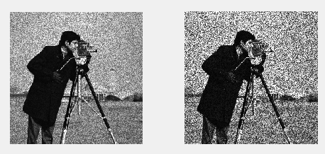

9.产生均匀分布的噪声

close all; clear all; clc; 

m = 256; 
n = 256; 
a = 50;
b = 180; 
I = a + (b - a) * rand(m, n); 

figure; 
subplot(121), imshow(uint8(I)); 
subplot(122), imhist(uint8(I));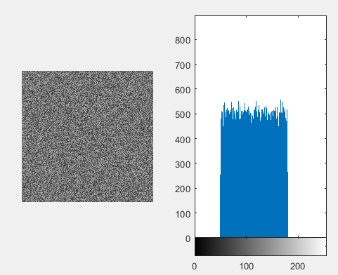

10.产生指数分布的噪声

close all; clear all; clc; 

m = 256; 
n = 256; 
a = 0.04; 
k = -1/a; 
I = k * log(1 - rand(m, n)); 

figure; 
subplot(121), imshow(uint8(I)); 
subplot(122), imhist(uint8(I)); 
axis tight;

11.对图像进行算术均值和几何均值滤波

close all; clear all; clc; 

I = im2double(imread('cameraman.tif'));
I = imnoise(I, 'gaussian', 0.05); 

w = fspecial('average', 3); 
J = imfilter(I, w); % 算术均值滤波
K = exp(imfilter(log(I), w)); % 几何均值滤波

figure; 
subplot(131), imshow(I); 
subplot(132), imshow(J);
subplot(133), imshow(K);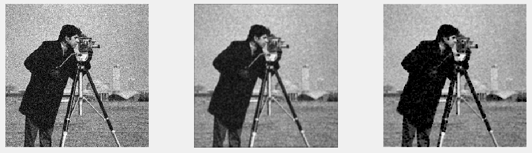

12.采用逆谐波均值滤波器对图像进行滤波

Q为滤波器的阶数。当Q为正数时，该滤波器可以去除椒噪声；当Q为负数时，该滤波器可以去除盐噪声。但是，该滤波器不能同时去除椒噪声和盐噪声。当Q=-1时，该滤波器为谐波均值滤波器。

close all; clear all; clc; 

I = im2double(imread('cameraman.tif'));
I = imnoise(I, 'salt & pepper', 0.01); % 添加密度为0.05的椒盐噪声

w = fspecial('average', 3); 
Q1 = 1.6; 
Q2 = -1.6; 

j1 = imfilter(I .^ (Q1+1), w); 
j2 = imfilter(I .^ Q1, w); 
J = j1 ./ j2; 

k1 = imfilter(I .^ (Q2+1), w); 
k2 = imfilter(I .^ Q2, w); 
K = k1 ./ k2; 

figure; 
subplot(131), imshow(I); 
subplot(132), imshow(J);
subplot(133), imshow(K);

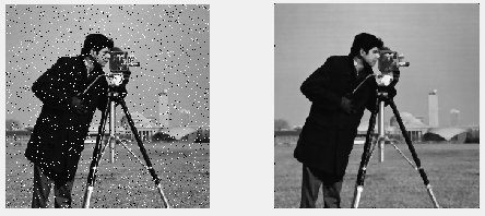
13.采用二维中值滤波对图像进行复原

close all; clear all; clc; 

I = im2double(imread('cameraman.tif'));
I = imnoise(I, 'salt & pepper', 0.05); % 添加密度为0.05的椒盐噪声

J = medfilt2(I, [3, 3]); 

figure; 
subplot(121), imshow(I); 
subplot(122), imshow(J);

14.采用二维排序滤波对图像进行复原

close all; clear all; clc; 

I = im2double(imread('cameraman.tif'));
I = imnoise(I, 'salt & pepper', 0.05); % 添加密度为0.05的椒盐噪声

domain = [0 1 1 0; 1 1 1 1; 1 1 1 1; 0 1 1 0]; % 窗口模板
J = ordfilt2(I, 6, domain); % 顺序滤波

figure; 
subplot(121), imshow(I); 
subplot(122), imshow(J);

15.采用最大值和最小值进行滤波复原

close all; clear all; clc; 

I = im2double(imread('cameraman.tif'));
I = imnoise(I, 'salt & pepper', 0.05); % 添加密度为0.05的椒盐噪声

J = ordfilt2(I, 1, ones(3)); % 选取最小值为像素值
K = ordfilt2(I, 9, ones(3)); % 选取最大值为像素值

figure; 
subplot(121), imshow(J); 
subplot(122), imshow(K);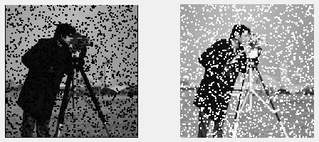

16.对图像进行自适应滤波

close all; clear all; clc; 

orginal_image = imread('saturn.png'); % 读取原彩色图像
I = rgb2gray(orginal_image);  % 灰度变换
I = imcrop(I, [100, 100, 1024, 1024]); % 剪切
J = imnoise(I, 'gaussian', 0, 0.03); % 加入高斯噪声
[K, noise] = wiener2(J, [5, 5]); % 自适应维纳滤波

figure; 
subplot(221), imshow(orginal_image); 
subplot(222), imshow(I); 
subplot(223), imshow(J); 
subplot(224), imshow(K);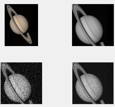

17.通过维纳滤波对运动模糊图像进行复原

close all; clear all; clc; 

I = imread('onion.png'); 
I = rgb2gray(I); 
I = im2double(I); 

LEN = 25; % 运动位移为25个像素
THETA = 20; % 角度为20°
PSF = fspecial('motion', LEN, THETA); % 产生点扩散函数PSF
J = imfilter(I, PSF, 'conv', 'circular');  % 运动模糊
NSR = 0; 
K = deconvwnr(J, PSF, NSR); % 维纳滤波复原

figure; 
subplot(131), imshow(I), title('原始图像'); 
subplot(132), imshow(J), title('运动模糊');
subplot(133), imshow(K), title('滤波图像');

【matlab代码练习14】图像复原技术

猜你喜欢