链接: 【数字图像处理】实验(1)——图像基本变换
链接: 【数字图像处理】实验(2)——图像增强(MATLAB实现)
链接: 【数字图像处理】实验(3)——图像综合应用:皮肤美化(MATLAB实现)
图像复原及几何校正
一、实验目的
(1)理解退化模型。
(2)掌握常用的图像复原方法。
二、实验原理
1.灰度线性变换就是将图像中所有点的灰度按照线性灰度变换函数进行变换。
2.直方图均衡化通过点运算将输入图像转换为在每一级上都有相等像素点数的输出图像。
3. 在实际的成像系统中,图像捕捉介质平面和物体平面之间不可避免地存在有一定的转角和倾斜角。 转角对图像的影响是产生图像旋转,倾斜角的影响表现为图像发生投影变形。另外一种情况是由于摄像机系统本身的原因导致的镜头畸变。此外,还有由于物体本身平面不平整导致的曲面畸变如柱形畸变等。这些畸变统称为几何畸变。
4.图像插值是一种基本的图像处理方法,它可以为数字图像增加或减少像素的数目。 当图像被放大时,像素会相应地增加,该像素增加的过程实际就是插值程序自动选择信息较好的像素作为新的像素以弥补空白像素空间的过程。虽然经过插值后图像可以变得更平滑、干净,但由于新增加的像素也仅仅只是原始像素的某种组合而已,所以图像的插值运算并不会增加新的图像信息。
插值图像提供坐标–>计算该坐标在原始图像中的对应坐标–>原始图像返回像素值并进行插值运算双线性插值法充分利用了邻域像素的不同占比程度而计算得出最合适的插值像素,从而完成插值。相比较于最近邻插值,双线性插值的插值效果要好得多,因为最近邻插值只跟(x,y)最近的像素值有关,而双线性插值是按照(x,y)上下、左右四个像素值的重要程度进行插值的(即越接近越重要)。
5.维纳(wiener)滤波 可以归于反卷积(或反转滤波)算法一类,它是由Wiener首提出的,并应用于一维信号,并取得很好的效果。以后算法又被引入二维信号理,也取得相当满意的效果,尤其在图象复原领域,由于维纳滤波器的复原效良好,计算量较低,并且抗噪性能优良,因而在图象复原领域得到了广泛的应用并不断得到改进发展,许多高效的复原算法都是以此为基础形成的。
三、实验步骤(包括分析、代码和波形)
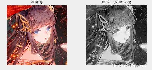
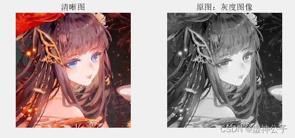
1. 选择一幅清晰的灰度图像,对该图像进行模糊化处理并加入高斯噪声,然后分别采用逆滤波、维纳滤波和约束最小二乘方滤波对模糊图像进行复原,比较各种图像复原方法的复原效果。
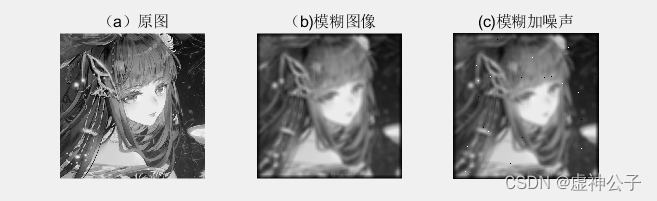
(1)对该图像进行模糊化处理并加入高斯噪声
代码:
%1.对该图像进行模糊化处理并加入高斯噪声
clear,clc,close all;
Image1=im2double(imread('lotus1.bmp'));
%figure,imshow(Image1),title('清晰图');
noiseIg=im2double(rgb2gray(imread('lotus1.bmp')));
%figure,imshow(noiseIg),title('原图:灰度图像');

figure;
subplot(121),imshow(Image1),title('清晰图');
subplot(122),imshow(noiseIg),title('原图:灰度图像');

%1.1 对该图像进行模糊化处理
L=20;theta=60;                                %运动模糊参数,30°方向上移动20个像素
halfL = (L-1)/2;                                %运动长度的一半,半个模板的对角长度
phi = mod(theta,180)/180*pi;
cosphi = cos(phi);    sinphi = sin(phi);
xsign = sign(cosphi);
linewdt = 1;                                    %运动方向上像素在线宽为1的范围内
halfhw = fix(halfL*cosphi + linewdt*xsign-eps);       %半个运动模糊模板宽
halphh = fix(halfL*sinphi + linewdt-eps);             %半个运动模糊模板高
[x,y] = meshgrid(0:xsign:halfhw, 0:halphh);           %半个模板中x、y坐标变化范围
dist2line = (y*cosphi-x*sinphi);                     %计算y',或称之为点到运动方向的距离
rad = sqrt(x.^2 + y.^2);                            %半个模板的对角长度
lastpix = find((rad >= halfL)&(abs(dist2line)<=linewdt)); % 在线宽范围内但超出运动长度的点
x2lastpix = halfL - abs((x(lastpix) + dist2line(lastpix)*sinphi)/cosphi);
dist2line(lastpix) = sqrt(dist2line(lastpix).^2 + x2lastpix.^2); %计算超范围的点到运动方向前端点的距离
dist2line = linewdt + eps - abs(dist2line);             %各点在模板中的权值,其总和约为L
dist2line(dist2line<0) = 0;                         %在距离运动方向线宽内的点保留,其余置零
h = rot90(dist2line,2);
h(end+(1:end)-1,end+(1:end)-1) = dist2line;           %将模板旋转180°,并补充完整
h = h./(sum(h(:)) + eps);                           %运动方向上
if cosphi>0
   h = flipud(h);
end
MotionBlurredI=conv2(h,noiseIg);
%figure,imshow(MotionBlurredI),title('模糊化处理');

%1.2 加入高斯噪声
noiseIg=imnoise(MotionBlurredI,'gaussian');
result2=medfilt2(noiseIg);
%figure,imshow(noiseIg),title('模糊化处理并加入高斯噪声');

figure;
subplot(121),imshow(MotionBlurredI),title('模糊化处理');
subplot(122),imshow(noiseIg),title('模糊化处理并加入高斯噪声');
结果:

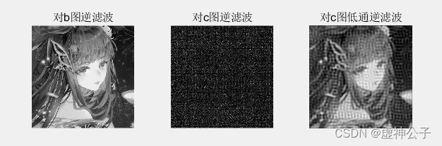
(2)逆滤波复原
代码:
clear,clc,close all;
noiseIg=im2double(rgb2gray(imread('lotus1.bmp')));
window=15;
[n,m]=size(noiseIg);
n=n+window-1;

m=m+window-1;
h=fspecial('average',window);
BlurI=conv2(h,noiseIg);
BlurandnoiseI=imnoise(BlurI,'salt & pepper',0.001);
%figure,imshow(noiseIg),title('(a)原图');
%figure,imshow(BlurI),title('(b)模糊图像');
%figure,imshow(BlurandnoiseI),title('(c)模糊加噪声');
figure;
subplot(131),imshow(noiseIg),title('(a)原图');
subplot(132),imshow(BlurI),title('(b)模糊图像');
subplot(133),imshow(BlurandnoiseI),title('(c)模糊加噪声');

imwrite(BlurI,'Blurred.jpg');
imwrite(BlurandnoiseI,'blurrednoise.jpg');

h1=zeros(n,m);
h1(1:window,1:window)=h;
H=fftshift(fft2(h1));
H(abs(H)<0.0001)=0.01;
M=H.^(-1);
r1=floor(m/2);  r2=floor(n/2);d0=sqrt(m^2+n^2)/20;
for u=1:m
    for v=1:n
        d=sqrt((u-r1)^2+(v-r2)^2);
        if d>d0
            M(v,u)=0;
        end
    end
end

G1=fftshift(fft2(BlurI));
G2=fftshift(fft2(BlurandnoiseI));

f1=ifft2(ifftshift(G1./H));
f2=ifft2(ifftshift(G2./H));
f3=ifft2(ifftshift(G2.*M));

result1=f1(1:n-window+1,1:m-window+1);
result2=f2(1:n-window+1,1:m-window+1);
result3=f3(1:n-window+1,1:m-window+1);

%figure,imshow(abs(result1),[]),title('对b图逆滤波');
%figure,imshow(abs(result2),[]),title('对c图逆滤波');
%figure,imshow(abs(result3),[]),title('对c图低通逆滤波');

imwrite(abs(result1),'Filteredimage1.jpg');
imwrite(abs(result2),'Filteredimage2.jpg');
imwrite(abs(result3),'Filteredimage3.jpg');

figure;
subplot(131),imshow(abs(result1),[]),title('对b图逆滤波');
subplot(132),imshow(abs(result2),[]),title('对c图逆滤波');
subplot(133),imshow(abs(result3),[]),title('对c图低通逆滤波');
结果:
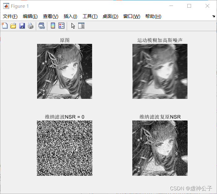
(3)维纳滤波复原
代码:
clear,clc,close all;
Image=im2double(rgb2gray(imread('lotus1.bmp')));
%3.维纳滤波
noiseIg=im2double(rgb2gray(imread('lotus1.bmp')));
subplot(221),imshow(noiseIg),title('原图');

LEN=21;
THETA=11;
PSF=fspecial('motion', LEN, THETA);
BlurredI=imfilter(noiseIg, PSF, 'conv', 'circular');

noise_mean = 0;
noise_var = 0.0001;
BlurandnoisyI=imnoise(BlurredI, 'gaussian', noise_mean, noise_var);
subplot(222), imshow(BlurandnoisyI),title('运动模糊加高斯噪声');
imwrite(BlurandnoisyI,'sbn.jpg');

estimated_nsr = 0;
result1= deconvwnr(BlurandnoisyI, PSF, estimated_nsr);
subplot(223),imshow(result1),title('维纳滤波NSR = 0');
imwrite(result1,'runsr0.jpg');

estimated_nsr = noise_var / var(Image(:));
result2 = deconvwnr(BlurandnoisyI, PSF, estimated_nsr);
subplot(224),imshow(result2),title('维纳滤波复原NSR');
imwrite(result2,'ruensr.jpg');
截图:
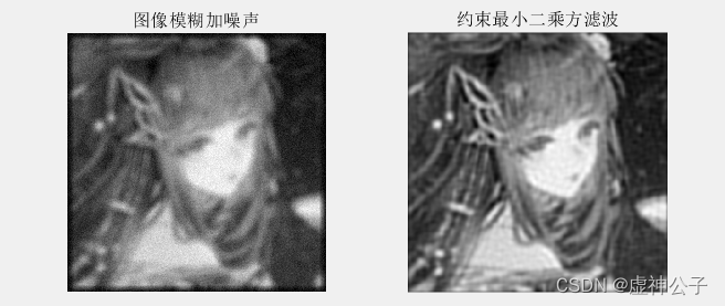
(4)约束最小二乘方滤波复原
代码:
clear,clc,close all;
noiseIg=im2double(rgb2gray(imread('lotus1.bmp')));
window=15;
[N,M]=size(noiseIg);
N=N+window-1;
M=M+window-1;
h=fspecial('average',window);
BlurI=conv2(h,noiseIg);
sigma=0.001;
miun=0;
nn=M*N*(sigma+miun*miun);
BlurandnoiseI=imnoise(BlurI,'gaussian',miun,sigma);
%figure,imshow(BlurandnoiseI),title('Blurred Image with noise');
figure;
subplot(121),imshow(BlurandnoiseI),title('图像模糊加噪声');
%imwrite(BlurandnoiseI,'Blurrednoiseimage.jpg');

h1=zeros(N,M);
h1(1:window,1:window)=h;
H=fftshift(fft2(h1));

lap=[0 1 0;1 -4 1;0 1 0];
L=zeros(N,M);
L(1:3,1:3)=lap;
L=fftshift(fft2(L));

G=fftshift(fft2(BlurandnoiseI));
gama=0.3;
step=0.01;
alpha=nn*0.001;
flag=true;
while flag
    MH=conj(H)./(abs(H).^2+gama*(abs(L).^2));
    F=G.*MH;
    E=G-H.*F;
    E=abs(ifft2(ifftshift(E)));
    ee=sum(E(:).^2);
    if ee<nn-alpha
        gama=gama+step;
    elseif ee>nn+alpha
        gama=gama-step;
    else
        flag=false;
    end
end
MH=conj(H)./(abs(H).^2+gama*(abs(L).^2));
f=ifft2(ifftshift(G.*MH));
result=f(1:N-window+1,1:M-window+1);
[J, LAGRA]=deconvreg(BlurandnoiseI,h,nn);

%figure,imshow(J,[]);

subplot(122),imshow(abs(result),[]),title('约束最小二乘方滤波');
%figure,imshow(abs(result),[]),title('Filtered Image');
imwrite(abs(result),'LSFilteredimage.jpg');
结果:
(5)整体代码
%1.对该图像进行模糊化处理并加入高斯噪声
clear,clc,close all;
Image1=im2double(imread('lotus1.bmp'));
%figure,imshow(Image1),title('清晰图');
noiseIg=im2double(rgb2gray(imread('lotus1.bmp')));
%figure,imshow(noiseIg),title('原图:灰度图像');

figure;
subplot(121),imshow(Image1),title('清晰图');
subplot(122),imshow(noiseIg),title('原图:灰度图像');

%1.1 对该图像进行模糊化处理
L=20;theta=60;                                %运动模糊参数,30°方向上移动20个像素
halfL = (L-1)/2;                                %运动长度的一半,半个模板的对角长度
phi = mod(theta,180)/180*pi;
cosphi = cos(phi);    sinphi = sin(phi);
xsign = sign(cosphi);
linewdt = 1;                                    %运动方向上像素在线宽为1的范围内
halfhw = fix(halfL*cosphi + linewdt*xsign-eps);       %半个运动模糊模板宽
halphh = fix(halfL*sinphi + linewdt-eps);             %半个运动模糊模板高
[x,y] = meshgrid(0:xsign:halfhw, 0:halphh);           %半个模板中x、y坐标变化范围
dist2line = (y*cosphi-x*sinphi);                     %计算y',或称之为点到运动方向的距离
rad = sqrt(x.^2 + y.^2);                            %半个模板的对角长度
lastpix = find((rad >= halfL)&(abs(dist2line)<=linewdt)); % 在线宽范围内但超出运动长度的点
x2lastpix = halfL - abs((x(lastpix) + dist2line(lastpix)*sinphi)/cosphi);
dist2line(lastpix) = sqrt(dist2line(lastpix).^2 + x2lastpix.^2); %计算超范围的点到运动方向前端点的距离
dist2line = linewdt + eps - abs(dist2line);             %各点在模板中的权值,其总和约为L
dist2line(dist2line<0) = 0;                         %在距离运动方向线宽内的点保留,其余置零
h = rot90(dist2line,2);
h(end+(1:end)-1,end+(1:end)-1) = dist2line;           %将模板旋转180°,并补充完整
h = h./(sum(h(:)) + eps);                           %运动方向上
if cosphi>0
   h = flipud(h);
end
MotionBlurredI=conv2(h,noiseIg);
%figure,imshow(MotionBlurredI),title('模糊化处理');

%1.2 加入高斯噪声
noiseIg=imnoise(MotionBlurredI,'gaussian');
result2=medfilt2(noiseIg);
%figure,imshow(noiseIg),title('模糊化处理并加入高斯噪声');

figure;
subplot(121),imshow(MotionBlurredI),title('模糊化处理');
subplot(122),imshow(noiseIg),title('模糊化处理并加入高斯噪声');


% imwrite(MotionBlurredI,'MotionBlurredI.jpg');
%2.逆滤波
noiseIg=im2double(rgb2gray(imread('lotus1.bmp')));
window=15;
[n,m]=size(noiseIg);
n=n+window-1;

m=m+window-1;
h=fspecial('average',window);
BlurI=conv2(h,noiseIg);
BlurandnoiseI=imnoise(BlurI,'salt & pepper',0.001);
%figure,imshow(noiseIg),title('(a)原图');
%figure,imshow(BlurI),title('(b)模糊图像');
%figure,imshow(BlurandnoiseI),title('(c)模糊加噪声');
figure;
subplot(131),imshow(noiseIg),title('(a)原图');
subplot(132),imshow(BlurI),title('(b)模糊图像');
subplot(133),imshow(BlurandnoiseI),title('(c)模糊加噪声');

imwrite(BlurI,'Blurred.jpg');
imwrite(BlurandnoiseI,'blurrednoise.jpg');

h1=zeros(n,m);
h1(1:window,1:window)=h;
H=fftshift(fft2(h1));
H(abs(H)<0.0001)=0.01;
M=H.^(-1);
r1=floor(m/2);  r2=floor(n/2);d0=sqrt(m^2+n^2)/20;
for u=1:m
    for v=1:n
        d=sqrt((u-r1)^2+(v-r2)^2);
        if d>d0
            M(v,u)=0;
        end
    end
end

G1=fftshift(fft2(BlurI));
G2=fftshift(fft2(BlurandnoiseI));

f1=ifft2(ifftshift(G1./H));
f2=ifft2(ifftshift(G2./H));
f3=ifft2(ifftshift(G2.*M));

result1=f1(1:n-window+1,1:m-window+1);
result2=f2(1:n-window+1,1:m-window+1);
result3=f3(1:n-window+1,1:m-window+1);

%figure,imshow(abs(result1),[]),title('对b图逆滤波');
%figure,imshow(abs(result2),[]),title('对c图逆滤波');
%figure,imshow(abs(result3),[]),title('对c图低通逆滤波');

imwrite(abs(result1),'Filteredimage1.jpg');
imwrite(abs(result2),'Filteredimage2.jpg');
imwrite(abs(result3),'Filteredimage3.jpg');

figure;
subplot(131),imshow(abs(result1),[]),title('对b图逆滤波');
subplot(132),imshow(abs(result2),[]),title('对c图逆滤波');
subplot(133),imshow(abs(result3),[]),title('对c图低通逆滤波');

%3.维纳滤波
noiseIg=im2double(rgb2gray(imread('lotus1.bmp')));
subplot(221),imshow(noiseIg),title('原图');

LEN=21;
THETA=11;
PSF=fspecial('motion', LEN, THETA);
BlurredI=imfilter(noiseIg, PSF, 'conv', 'circular');

noise_mean = 0;
noise_var = 0.0001;
BlurandnoisyI=imnoise(BlurredI, 'gaussian', noise_mean, noise_var);
subplot(222), imshow(BlurandnoisyI),title('运动模糊加高斯噪声');
imwrite(BlurandnoisyI,'sbn.jpg');

estimated_nsr = 0;
result1= deconvwnr(BlurandnoisyI, PSF, estimated_nsr);
subplot(223),imshow(result1),title('维纳滤波NSR = 0');
imwrite(result1,'runsr0.jpg');

estimated_nsr = noise_var / var(noiseIg(:));
result2 = deconvwnr(BlurandnoisyI, PSF, estimated_nsr);
subplot(224),imshow(result2),title('维纳滤波复原NSR');
imwrite(result2,'ruensr.jpg');

%4.约束最小二乘方滤波
noiseIg=im2double(rgb2gray(imread('lotus1.bmp')));
window=15;
[N,M]=size(noiseIg);
N=N+window-1;
M=M+window-1;
h=fspecial('average',window);
BlurI=conv2(h,noiseIg);
sigma=0.001;
miun=0;
nn=M*N*(sigma+miun*miun);
BlurandnoiseI=imnoise(BlurI,'gaussian',miun,sigma);
%figure,imshow(BlurandnoiseI),title('Blurred Image with noise');
figure;
subplot(121),imshow(BlurandnoiseI),title('图像模糊加噪声');
%imwrite(BlurandnoiseI,'Blurrednoiseimage.jpg');

h1=zeros(N,M);
h1(1:window,1:window)=h;
H=fftshift(fft2(h1));

lap=[0 1 0;1 -4 1;0 1 0];
L=zeros(N,M);
L(1:3,1:3)=lap;
L=fftshift(fft2(L));

G=fftshift(fft2(BlurandnoiseI));
gama=0.3;
step=0.01;
alpha=nn*0.001;
flag=true;
while flag
    MH=conj(H)./(abs(H).^2+gama*(abs(L).^2));
    F=G.*MH;
    E=G-H.*F;
    E=abs(ifft2(ifftshift(E)));
    ee=sum(E(:).^2);
    if ee<nn-alpha
        gama=gama+step;
    elseif ee>nn+alpha
        gama=gama-step;
    else
        flag=false;
    end
end
MH=conj(H)./(abs(H).^2+gama*(abs(L).^2));
f=ifft2(ifftshift(G.*MH));
result=f(1:N-window+1,1:M-window+1);
[J, LAGRA]=deconvreg(BlurandnoiseI,h,nn);

%figure,imshow(J,[]);

subplot(122),imshow(abs(result),[]),title('约束最小二乘方滤波');
%figure,imshow(abs(result),[]),title('Filtered Image');
imwrite(abs(result),'LSFilteredimage.jpg');
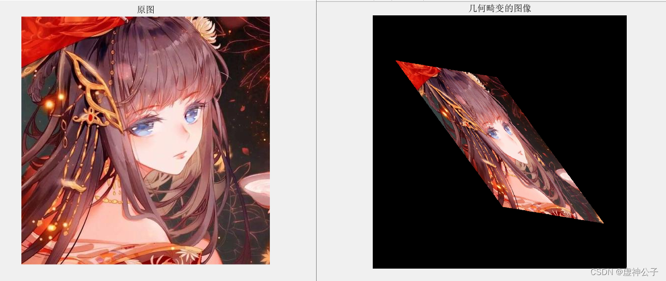
2. 选择一幅清晰的灰度图像,对该图像进行仿射变换(maketform,imtransform),然后分别采用连接点选择、空间变换和灰度插值对几何失真的图像进行复原,比较各种图像复原方法的复原效果。
(1)对该图像进行仿射变换(maketform,imtransform)
代码:
%1.对该图像进行模糊化处理
clear,clc,close all;
Image1=im2double(imread('lotus1.bmp'));
%figure,imshow(Image1),title('清晰图');
noiseIg=im2double(rgb2gray(imread('lotus1.bmp')));
%figure,imshow(noiseIg),title('原图:灰度图像');

figure;
subplot(121),imshow(Image1),title('清晰图');
subplot(122),imshow(noiseIg),title('原图:灰度图像');


%1.对该图像进行仿射变换(maketform,imtransform)
Image=im2double(imread('lotus1.bmp'));
[h,w,c]=size(Image);
figure,imshow(Image),title('原图');
RI=imrotate(Image,20);
tform=maketform('affine',[1 0.5 0;0.5 1 0; 0 0 1]);
NewImage=imtransform(RI,tform);
figure,imshow(NewImage),title('几何畸变的图像');
imwrite(NewImage,'GDImage.jpg');
cpselect(NewImage,Image);
结果:
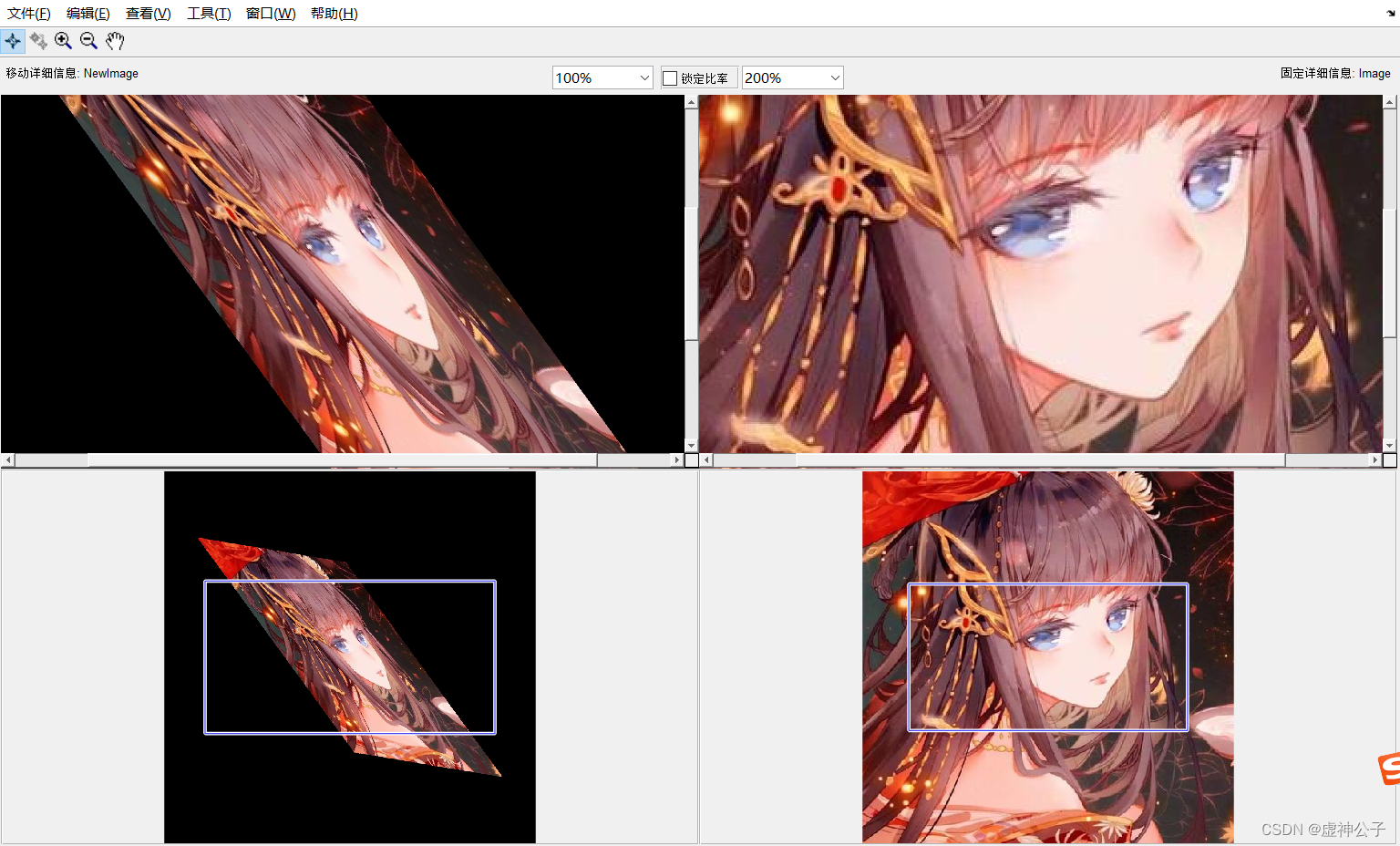
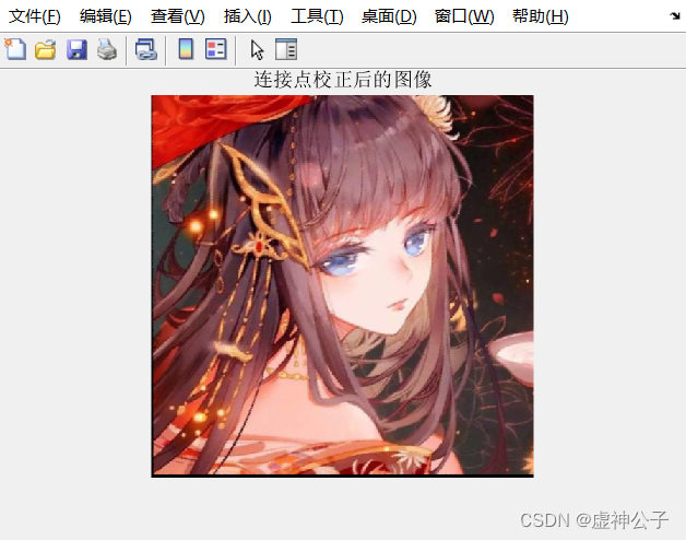
(2)连接点选择复原
代码:
%2.连接点选择
input_points=[709 577;409 270;320 370];
base_points=[487 305;374 41;134 159];
tform=cp2tform(input_points,base_points,'affine');
%几何变换
result=imtransform(NewImage,tform,'XData',[1 w],'YData',[1 h]);
figure,imshow(result),title('连接点校正后的图像');
imwrite(result,'jiaozheng.jpg');
结果:
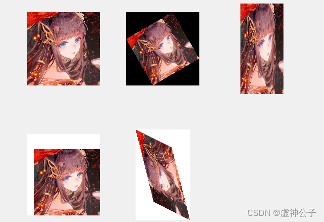
(3)空间变换复原
代码:
%3.空间变换
I=im2double(imread('lotus1.bmp'));

%实现图像旋转
Ia = maketform('affine', [cosd(30) -sind(30) 0; sind(30) cosd(30) 0; 0 0 1]);
Ia = imtransform(I, Ia);

%实现图像缩放
Ib = maketform('affine', [5 0 0; 0 10.5 0; 0 0 1]);
Ib = imtransform(I, Ib);

%实现图像平移
xform = [1 0 55; 0 1 115; 0 0 1]';
Ic = maketform('affine', xform);
Ic = imtransform(I, Ic, 'XData', ...
    [1 (size(I, 2) + xform(3, 1))], 'YData', ...
    [1 (size(I, 1) + xform(3, 2))], 'FillValues', 255);

%实现图像整体切变
Id = maketform('affine', [1 4 0; 2 1 0; 0 0 1]);
Id = imtransform(I, Id, 'FillValues', 255);

figure;
subplot(231);imshow(I);	 %显示原图像
subplot(232);imshow(Ia); %旋转
subplot(233);imshow(Ib); %缩放
subplot(234);imshow(Ic); %平移
subplot(235);imshow(Id); %整体切变
结果:
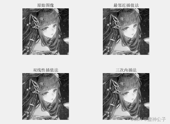
(4)灰度插值复原
代码:
%4.灰度插值
I=im2double(imread('lotus1.bmp'));
I=rgb2gray(I);%将真彩色图像转换为灰度图像;
X1=imresize(I,1);%采用最邻近插值法进行灰度插值;
X2=imresize(I,1,'bilinear');%采用双线性插值法进行灰度插值;
X3=imresize(I,1,'bicubic');%采用三次内插法进行灰度插值;
subplot(221),imshow(I,[ ]),title('原始图像');
subplot(222),imshow(X1),title('最邻近插值法');
subplot(223),imshow(X2),title('双线性插值法');
subplot(224),imshow(X3),title('三次内插法');
结果:
(5)整体代码
代码:
%1.对该图像进行模糊化处理
clear,clc,close all;
Image1=im2double(imread('lotus1.bmp'));
%figure,imshow(Image1),title('清晰图');
noiseIg=im2double(rgb2gray(imread('lotus1.bmp')));
%figure,imshow(noiseIg),title('原图:灰度图像');

figure;
subplot(121),imshow(Image1),title('清晰图');
subplot(122),imshow(noiseIg),title('原图:灰度图像');


%1.对该图像进行仿射变换(maketform,imtransform)
Image=im2double(imread('lotus1.bmp'));
[h,w,c]=size(Image);
figure,imshow(Image),title('原图');
RI=imrotate(Image,20);
tform=maketform('affine',[1 0.5 0;0.5 1 0; 0 0 1]);
NewImage=imtransform(RI,tform);
figure,imshow(NewImage),title('几何畸变的图像');
imwrite(NewImage,'GDImage.jpg');
cpselect(NewImage,Image);

%2.连接点选择
input_points=[709 577;409 270;320 370];
base_points=[487 305;374 41;134 159];
tform=cp2tform(input_points,base_points,'affine');
%几何变换
result=imtransform(NewImage,tform,'XData',[1 w],'YData',[1 h]);
figure,imshow(result),title('连接点校正后的图像');
imwrite(result,'jiaozheng.jpg');

%3.空间变换
I=im2double(imread('lotus1.bmp'));

%实现图像旋转
Ia = maketform('affine', [cosd(30) -sind(30) 0; sind(30) cosd(30) 0; 0 0 1]);
Ia = imtransform(I, Ia);

%实现图像缩放
Ib = maketform('affine', [5 0 0; 0 10.5 0; 0 0 1]);
Ib = imtransform(I, Ib);

%实现图像平移
xform = [1 0 55; 0 1 115; 0 0 1]';
Ic = maketform('affine', xform);
Ic = imtransform(I, Ic, 'XData', ...
    [1 (size(I, 2) + xform(3, 1))], 'YData', ...
    [1 (size(I, 1) + xform(3, 2))], 'FillValues', 255);

%实现图像整体切变
Id = maketform('affine', [1 4 0; 2 1 0; 0 0 1]);
Id = imtransform(I, Id, 'FillValues', 255);

figure;
subplot(231);imshow(I);	 %显示原图像
subplot(232);imshow(Ia); %旋转
subplot(233);imshow(Ib); %缩放
subplot(234);imshow(Ic); %平移
subplot(235);imshow(Id); %整体切变


%4.灰度插值
I=im2double(imread('lotus1.bmp'));
I=rgb2gray(I);%将真彩色图像转换为灰度图像;
X1=imresize(I,1);%采用最邻近插值法进行灰度插值;
X2=imresize(I,1,'bilinear');%采用双线性插值法进行灰度插值;
X3=imresize(I,1,'bicubic');%采用三次内插法进行灰度插值;
subplot(221),imshow(I,[ ]),title('原始图像');
subplot(222),imshow(X1),title('最邻近插值法');
subplot(223),imshow(X2),title('双线性插值法');
subplot(224),imshow(X3),title('三次内插法');
四、实验总结
1.典型的图像复原方法及其适用范围
逆滤波:适用于无噪声图像,一般对于有噪声的图像来说,直接逆滤波的性能是较差的。
最小均方差滤波(维纳)滤波:该方法建立在图像和噪声都是随机变量的基础上。未退化图像和噪声的功率谱必须是已知的。在没有噪声的情况下,维纳滤波可以看作是逆滤波。
约束最小二乘方滤波:仅仅用噪声的均值和方差的知识,就可以实现的最佳复原算法。但要假设噪声和图像灰度值不相关。
几何均值滤波:对维纳滤波的推广。
投影重建图像,卡尔曼滤波等。图像复原算法有线性和非线性两类。线性算法通过对图像进行逆滤波来实现反卷积。非线性方法通过连续的迭代过程不断提高复原质量,直到满足预先设定的终止条件,结果往往令人满意。
2.Matlab空间变换函数 imtransform
可以实现图像仿射变换(如 平移、旋转、剪切、缩放)、投影变换, 该函数可与 maketform 配合使用。不过官网目前更推荐使用 imwarp
用法说明:
B = imtransform(A,tform)
根据 tform 定义的二维空间变换来变换图像 A,并返回变换后的图像 B。如果 A 是彩色图像,则 imtransform 会对每个颜色通道应用相同的二维变换。类似地,如果 A 是三维体或具有三个或更多维度的图像序列,则 imtransform 将相同的二维变换应用于沿更高维度的所有二维平面。对于任意维度的数组变换,请使用 tformarray。
B = imtransform(A,tform,interp)
指定要使用的插值形式。
B = imtransform(,Name,Value)
使用名称-值对组来控制空间变换的各个方面。
[B,xdata,ydata] = imtransform()
还返回输出图像 B 在输出 X-Y 空间中的范围。默认情况下,imtransform 会自动计算 xdata 和 ydata,使得 B 包含整个变换后的图像 A。但是,您可以通过为 XData 和 YData 名称-值对组输入参数指定值来覆盖此自动计算