python一对一辅导教程：PyGeM Tutorials 解析 1

作者自我介绍：大爽歌, b站小UP主 ，直播编程+红警三 ，python1对1辅导老师 。
本博客为一对一辅导学生python代码的教案, 获得学生允许公开。
目前具体辅导内容为PyGeM

本文为PyGeM tutorial-1-ffd 的讲解与分析
Tutorial 1 shows how to apply the free-form deformation to mesh nodes.

0 准备工作

准备软件

必须安装

1. python 3.8或以上版本
   https://www.python.org/downloads/
2. conda
   conda 又分为 Anaconda 和 Miniconda
   电脑性能足够好，推荐安装 Anaconda (这个是一个很大的软件)
   性能一般或者不想安装太多太大的东西，可以尝试安装 Miniconda
   Anaconda: https://www.anaconda.com/products/individual
   Miniconda: https://docs.conda.io/en/latest/miniconda.html

推荐安装
3. Pycharm
https://blog.csdn.net/python1639er/article/details/122629870

安装第三方库 pygem

PyGeM 不能直接使用pip来安装，需要按如下步骤来。 (准确来讲，是pip安装的不符合需求，版本太老)

推荐先使用Pycharm建立项目，
再在Pycharm的Terminal中安装。(这个也相当于命令行)
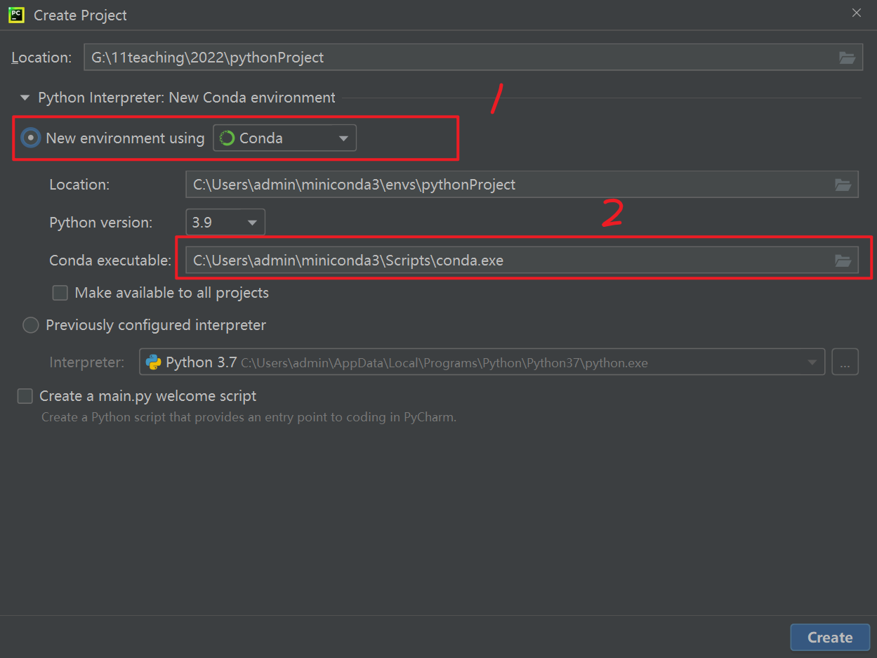
Pycharm 建立项目时 Python Interpreter建议选择如下

1选Conda
2根据自己电脑上Conda的位置来选

先安装依赖库

1. 可以直接pip安装的有
   numpy, scipy, matplotlib, sphinx, pytest
   安装命令如下(命令行中运行)

pip install numpy
pip install scipy
pip install matplotlib
pip install sphinx
pip install pytest

安装不上可能需要使用镜像，
具体推荐阅读:
大爽Python入门教程 8-2 Python 库(Library)、包(Package)、模块(Module) 的第三方库部分。

2. 手动安装 pythonocc-core
   要使用子模块submodule，则需要安装这个。
   可以使用conda命令来安装
   安装命令如下(命令行中运行)

conda install -c conda-forge pythonocc-core=7.4.0

3. 手动安装 PyGeM

安装命令如下(命令行中运行)

git clone https://github.com/mathLab/PyGeM

然后将控制台当前路径切换到这个项目的文件夹中去
如果在Pycharm的项目的Terminal 中运行的上面的代码的话，
这时Terminal切换路径的命令为

cd PyGeM

然后输入以下命令即可安装PyGeM

python setup.py install

到这里基本就安装好了

1 开头

首段

原文与翻译

Free Form Deformation on a sphere
球体上的自由形式变形
In this tutorial we will show the typical workflow to perform a deformation on a generic geometry using the free-form deformation method implemented within PyGeM.
在本教程中，我们将展示使用 PyGeM 中实现的自由形式变形(FFD)方法对通用几何图形执行变形的典型工作流程。
A brief theoretical overview of the method is introduced in the pygem.ffd module,
pygem.ffd 模块中介绍了该方法的简要理论概述，
while in the README you can find several references that focus on FFD.
而在README中，您可以找到一些关注 FFD 的参考资料。

First of all, we import the required PyGeM class and we set matplotlib for 3D plots.
首先，我们导入所需的 PyGeM 类，并为 3D 绘图设置 matplotlib。
The version of PyGeM we are using in this tutorial is the 2.0.0.
我们在本教程中使用的 PyGeM 版本是 2.0.0。

导入

原文代码

%matplotlib inline
import numpy as np
import mpl_toolkits.mplot3d
import matplotlib.pyplot as plt

import pygem
print(pygem.__version__)
from pygem import FFD

首行的%matplotlib inline是给 Ipython 编译器用的(可以在网页中做内嵌画图)，
常常是Jupyter或colab 的ipynb笔记本会用到。

一般.py文件不需要这个命令，注释或者删掉最好。

大爽Python入门教程 8-1 导入import

import math
print(math.pi)

from math import pi
print(pi)

import math as m
print(m.pi)

2 mesh_points

Then, the other ingredient is the original geometry we want to deform.
然后，另一个成分是我们想要变形的原始几何体。
In this simple tutorial we just span some points around a sphere and morph their coordinates using the FFD class.
在这个简单的教程中，我们只是跨越一个球体周围的一些点，并使用 FFD 类改变它们的坐标。

def mesh_points(num_pts = 2000):
    indices = np.arange(0, num_pts, dtype=float) + 0.5

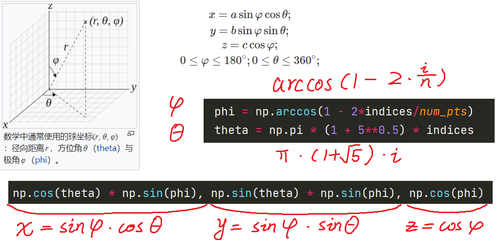
    phi = np.arccos(1 - 2*indices/num_pts)
    theta = np.pi * (1 + 5**0.5) * indices

    return np.array([np.cos(theta) * np.sin(phi), np.sin(theta) * np.sin(phi), np.cos(phi)]).T

mesh = mesh_points()
plt.figure(figsize=(8,8)).add_subplot(111, projection='3d').scatter(*mesh.T);
plt.show()

phi

numpy.arange(start, stop, dtype = None)
Return evenly spaced values within a given interval.
在给定的间隔内返回均匀间隔的值。

>>> import numpy as np
>>> np.arange(0, 5, dtype=float)
array([0., 1., 2., 3., 4.])
np.arange(0, 5, dtype=float) + 0.5
array([0.5, 1.5, 2.5, 3.5, 4.5])
>>> np.arange(0, 2000, dtype=float) + 0.5
array([5.0000e-01, 1.5000e+00, 2.5000e+00, ..., 1.9975e+03, 1.9985e+03,
       1.9995e+03])

关于e: 大爽Python入门教程 1-2 数与字符串

num_pts取默认值2000
indices = np.arange(0, 2000, dtype=float) + 0.5
得到了 0.5, 1.5, 2.5 一直到 1999.5 构成的数组

indices/num_pts 得到一个 1 分成 num_pts 份的数组
1 - 2* indices/num_pts得到一个[-1, 1]之间分成num_pts 份的数组

np.arccos(1 - 2*indices/num_pts)得到的是$[0,\pi ]$之间的的数构成的数组（此时不是均等分隔的了）
是如图y轴上均等分隔的点对应到曲线上的点的横坐标。

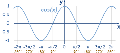
phi 对应球坐标系的$\varphi$
具体见后面的椭球公式

theta

np.pi * (1 + 5**0.5) * indices
这个就是$\pi \ast (1+\sqrt{5})$

这个是用于去得到坐标得，
采用得大概是黄金螺旋线法
详细原理我也不太明白，
这里就不深究了，能用就行。

感兴趣可以去看下这个:
evenly-distributing-n-points-on-a-sphere

return

np.array([np.cos(theta) * np.sin(phi), np.sin(theta) * np.sin(phi), np.cos(phi)])
会得到一个3行num_pts列的

[[ 0.05111927 -0.21801231  0.29980505 -0.19082906  ......  -0.17335079  0.14097948]
 [-0.13147935  0.10756687  0.08727502 -0.31414053  ......  0.17043915 -0.0049786 ]
 [ 0.99        0.97        0.95        0.93        ......  -0.97       -0.99      ]]

加个 .T得到 num_pts行3列的

[[ 0.05111927 -0.13147935  0.99      ]
 [-0.21801231  0.10756687  0.97      ]
 [ 0.29980505  0.08727502  0.95      ]
 [-0.19082906 -0.31414053  0.93      ]
 ......
 [-0.17335079  0.17043915 -0.97      ]
 [ 0.14097948 -0.0049786  -0.99      ]]

椭球公式

椭球

球坐标系，其中$\phi$是天顶角，$\theta$是方位角，则椭球可以表示为以下的参数形式：
$$\begin{gathered} x=a\sin \phi \cos \theta ; \\ y=b\sin \phi \sin \theta ; \\ z=c\cos \phi ; \\ 0\le \phi \le 180^{\circ };0\le \theta \le 360^{\circ }; \end{gathered}$$

3 第一张图

原文代码

import numpy as np
import matplotlib.pyplot as plt

def mesh_points(num_pts = 2000):
    indices = np.arange(0, num_pts, dtype=float) + 0.5

    phi = np.arccos(1 - 2*indices/num_pts)
    theta = np.pi * (1 + 5**0.5) * indices

    return np.array([np.cos(theta) * np.sin(phi), np.sin(theta) * np.sin(phi), np.cos(phi)]).T

mesh = mesh_points()
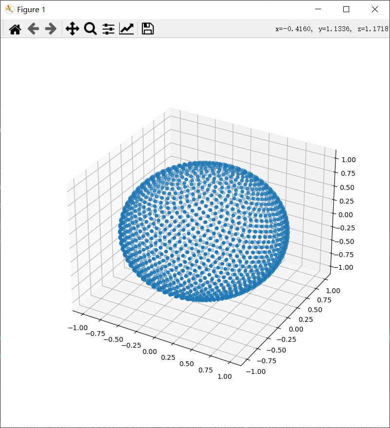
plt.figure(figsize=(8,8)).add_subplot(111, projection='3d').scatter(*mesh.T);
plt.show()

运行效果如图

这里来详细看下绘图部分代码

plt.figure(figsize=(8,8)).add_subplot(111, projection='3d').scatter(*mesh.T);
plt.show()

figure

plt.figure(figsize=(8,8))
Create a new figure, or activate an existing figure.
figsize 指定 Width, height in inches.

figure可以认为是绘图的窗口。

示例代码

import matplotlib.pyplot as plt
fig = plt.figure(figsize=(8,8))
plt.show()

运行效果如下

一个空的绘图窗口

subplot

该方法用于在窗口figure里面添加或规划轴线axes的

plt.subplot(*args, **kwargs)
Add an Axes to the current figure or retrieve an existing Axes.
将轴添加到当前图窗或检索现有轴。
This is a wrapper of Figure.add_subplot which provides additional behavior when working with the implicit API (see the notes section).
这是 Figure.add_subplot 的包装器，它在使用隐式 API 时提供额外的行为（请参阅注释部分）。

Call signatures:

subplot(nrows, ncols, index, **kwargs)  # 位置
subplot(pos, **kwargs)  # 位置
subplot(**kwargs)
subplot(ax)

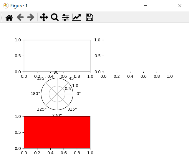
示例: tutorial_101d.py如下

import matplotlib.pyplot as plt

# 按 三行x二列 的布局分割窗口，
# 得到总共六块区域
# 在第1个区域，放下第1个轴线 ax1
# plt.subplot(321)
# 下面的和上面的效果相同，下面的写法更正式
ax1 = plt.subplot(3, 2, 1)

# 在第2个区域，放下第2个轴线 ax2
# 该轴线无边框
ax2 = plt.subplot(322, frameon=False)

# 在第3个区域，放下第3个轴线 ax3
# 该轴线为极坐标轴线
ax3 = plt.subplot(323, projection='polar')

# 在第4个区域，放下第4个轴线 ax4
# 该轴线背景色为红色
ax4 = plt.subplot(325, facecolor='red')

plt.show()

运行效果如下图

3d

fig.add_subplot(111, projection='3d')

• 111:在窗口中按一行x一列布局，在第一块区域放置轴线，
• projection='3d': 一个3d图轴线

实例代码

import matplotlib.pyplot as plt

fig = plt.figure(figsize=(8,8))
ax = fig.add_subplot(111, projection='3d')

plt.show()

运行效果如下图

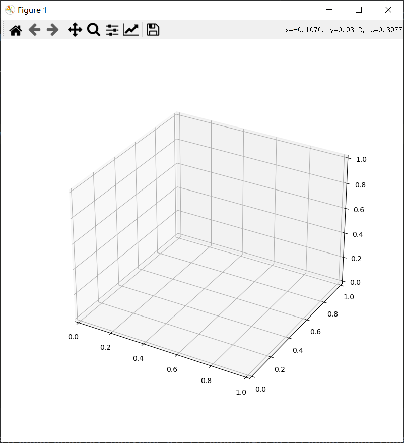
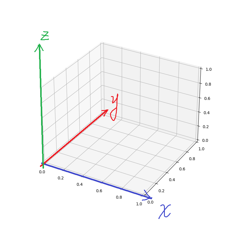
3d图的三轴具体如下

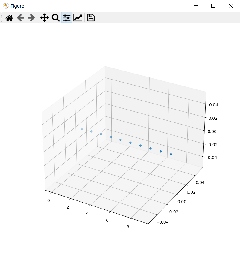
scatter

scatter(xs, ys, zs)
绘制散点图
根据指定的x, y, z 坐标

示例tutorial_101f.py如下

import matplotlib.pyplot as plt

fig = plt.figure(figsize=(8,8))

ax = fig.add_subplot(111, projection='3d')

xs = [i for i in range(10)]
ys = [0 for i in range(10)]
zs = [0 for i in range(10)]

ax.scatter(xs, ys, zs)

plt.show()

运行效果如下

绘图代码拆解

plt.figure(figsize=(8,8)).add_subplot(111, projection='3d').scatter(*mesh.T);

这一句长代码，拆解成一步一步的话，
等价于如下代码

fig = plt.figure(figsize=(8,8))
ax = fig.add_subplot(111, projection='3d')
xs, ys, zs = mesh.T
ax.scatter(xs, ys, zs)

还可以写成如下形式。

plt.figure(figsize=(8,8))
plt.add_subplot(111, projection='3d')
xs, ys, zs = mesh.T
plt.scatter(xs, ys, zs)