Lightly SSL 是一个用于自监督学习的计算机视觉框架。
github链接:GitHub - lightly-ai/lightly: A python library for self-supervised learning on images.
Documentation:Documentation — lightly 1.4.20 documentation
以下内容主要来自Documentation,部分内容省略,部分专业名字不翻译,主要复现教程6。
主要概念
Self-Supervised Learning
下图显示了 Lightly SSL 软件包所使用的不同概念概览,以及它们之间的交互模式。下文将对粗体表达式作进一步解释。

Dataset
在 Lightly SSL 中,数据集是通过 LightlyDataset 访问的。您可以从图像或视频目录创建一个 LightlyDataset,也可以直接从 torchvision 数据集创建一个 LightlyDataset。您可以在(教程1:构建输入)中了解更多相关信息:
- Tutorial 1: Structure Your Input (教程1:构建输入)
Transform
在自监督学习中,输入图像通常被随机转换成原始图像的视图。视图及其底层变换非常重要,因为它们定义了模型和图像 embedding 的属性。您既可以使用我们预定义的变换,也可以编写自己的变换。更多信息,请查看以下页面:
Collate Function
整理功能可将多个图像的视图汇总到一个批量中。您可以使用默认的整理函数。Lightly SSL 还提供了一个多视图校对函数MultiViewCollate
Dataloader
对于数据加载器,您可以简单地使用PyTorch dataloader。但一定要给它传递一个LightlyDataset!
Backbone Neural Network
自监督学习最酷的一点是,你可以预先训练你的神经网络,而无需标注数据。你可以插入任何你想要的 backbone!如果你不知道从哪里开始,可以看看我们的SimCLR示例,了解如何使用ResNet或 MSN 的 Vision Transformer backbone。
Heads
heads 是神经网络的最后一层,加在backbone之上。它们将backbone的输出(通常称为 embeddings、representations 或 features)投射到一个新的空间,并在其中计算损失。人们发现,这比直接计算 embedding 上的损失要有益得多。Lightly SSL 提供了可以添加到任何 backbone 中的常用heads。
Model
该模型将您的 backbone 神经网络与一个或多个heads 以及(如需要)动量编码器相结合,为最流行的自监督学习模型提供了一个易于使用的接口。我们的models 页面包含大量实现示例。如果你想了解更多关于模型和如何使用模型的信息,也可以浏览我们的教程:
- Tutorial 2: Train MoCo on CIFAR-10
- Tutorial 3: Train SimCLR on Clothing
- Tutorial 4: Train SimSiam on Satellite Images
Loss
损失函数在自监督学习中起着至关重要的作用。Lightly SSL 在loss 模块中提供了常见的损失函数。
Optimizer
使用 Lightly SSL,您可以使用任何 PyTorch optimizer 来训练模型。
Training
可以使用普通 PyTorch training loop或 PyTorch Lightning等专用框架来训练模型。Lightly SSL 可以让你选择最适合你的方式。请查看我们的 models 和tutorials 部分,了解如何使用 PyTorch 或 PyTorch Lightning 训练模型。
Image Embeddings
在训练过程中,模型学会从图像中创建紧凑的 embedding。这些 embedding(通常也称为表示或特征)可用于识别相似图像或从数据中创建多样化子集等任务:
Pre-Trained Backbone
自监督训练后,backbone 可以重复使用。它可用于任何其他需要类似网络架构的任务,包括图像分类、物体检测和分割任务。您可以在我们的物体检测教程中了解更多信息:
安装
Supported Python versions
Lightly SSL requires Python 3.6+. We recommend installing Lightly SSL in a Linux or OSX environment.
Installing Lightly SSL
You can install Lightly SSL and its dependencies from PyPi with:
pip install lightly
Dependencies
Lightly SSL 目前使用 PyTorch 作为底层深度学习框架。在 PyTorch 的基础上,我们使用Hydra来管理配置,使用 PyTorch Lightning来训练模型。
如果要处理视频文件,还需要额外安装 PyAV。
pip install av
教程1:构建输入
支持的文件类型
默认情况下,Lightly SSL Python 软件包可以处理图像或视频,用于自监督学习或生成嵌入。
Images
由于 Lightly SSL 使用 Pillow 来加载图片,因此它也支持 Pillow 支持的所有图片格式。
- .jpg, .png, .tiff and many more
Image Folder Datasets
图像文件夹数据集包含原始图像,通常使用 input_dir 关键字指定。
Flat Directory Containing Images
您可以将所有感兴趣的图片存储在一个文件夹中,而无需额外的层次结构。例如,Lightly SSL 将加载 data/. 目录中的所有文件名和图像。此外,它会为所有图片分配一个占位符标签。
# a single directory containing all images
data/
+--- img-1.jpg
+--- img-2.jpg
...
+--- img-N.jpg
对于上述结构,Lightly SSL 将按如下方式理解输入:
filenames = [
    'img-1.jpg',
    'img-2.jpg',
    ...
    'img-N.jpg',
]

labels = [
    0,
    0,
    ...
    0,
]
Directory with Subdirectories Containing Images
您可以将输入图像收集到子目录中,从而使输入目录结构化。在这种情况下,Lightly SSL 加载的文件名是相对于 "root directory "data/.的。此外,Lightly SSL 还会为每张图片分配一个所谓的 "weak-label",指明它属于哪个子目录。
# directory with subdirectories containing all images
data/
+-- weak-label-1/
    +-- img-1.jpg
    +-- img-2.jpg
    ...
    +-- img-N1.jpg
+-- weak-label-2/
    +-- img-1.jpg
    +-- img-2.jpg
    ...
    +-- img-N2.jpg
...
...
...
+-- weak-label-10/
    +-- img-1.jpg
    +-- img-2.jpg
    ...
    +-- img-N10.jpg
对于上面的结构,LightlySSL将理解输入如下:
filenames = [
    'weak-label-1/img-1.jpg',
    'weak-label-1/img-2.jpg',
    ...
    'weak-label-1/img-N1.jpg',
    'weak-label-2/img-1.jpg',
    ...
    'weak-label-2/img-N2.jpg',
    ...
    'weak-label-10/img-N10.jpg',
]

labels = [
    0,
    0,
    ...
    0,
    1,
    ...
    1,
    ...
    9,
]
教程2:在CIFAR-10上训练MoCo
在本教程中,我们将基于MoCo论文Momentum Contrast for Unsupervised Visual Representation Learnin训练一个模型。
在使用对比损失训练自监督模型时,我们通常会遇到一个大问题。为了获得良好的结果,我们需要大量的负示例来让对比损失发挥作用。因此,我们需要很大的批次规模。然而,并不是每个批次都能使用充满 GPU 或 TPU 的集群。为了解决这个问题,我们开发了其他方法。其中一些方法使用内存库来存储我们可以查询的旧负示例,以弥补较小的批次规模。MoCo 在此基础上更进一步,加入了动量编码器。
本教程使用 CIFAR-10 数据集。
在本教程中将学到:
- 如何使用轻量级加载数据集和训练模型
- 如何利用记忆库创建 MoCo 模型
- 如何在迁移学习任务中使用自监督学习后的预训练模型
Imports
导入本教程所需的 Python 框架。确保已经安装了lightly库。
import copy

import pytorch_lightning as pl
import torch
import torch.nn as nn
import torchvision

from lightly.data import LightlyDataset
from lightly.loss import NTXentLoss
from lightly.models import ResNetGenerator
from lightly.models.modules.heads import MoCoProjectionHead
from lightly.models.utils import (
    batch_shuffle,
    batch_unshuffle,
    deactivate_requires_grad,
    update_momentum,
)
from lightly.transforms import MoCoV2Transform, utils
Configuration
我们为实验设置了一些配置参数。请随意更改并分析其效果。
默认配置的batch size为 512。这需要大约 6.4GB 的 GPU 内存。在进行 100 次epochs训练时,测试集准确率应达到 73% 左右。当训练 200 个epochs时,准确率会提高到 80%。
num_workers = 8
batch_size = 512
memory_bank_size = 4096
seed = 1
max_epochs = 100
将路径替换为 CIFAR-10 数据集的位置。我们假设有一个 train 文件夹,里面有每个类的子文件夹和 .png 图像。
You can download CIFAR-10 in folders from Kaggle.
# The dataset structure should be like this:
# cifar10/train/
#  L airplane/
#    L 10008_airplane.png
#    L ...
#  L automobile/
#  L bird/
#  L cat/
#  L deer/
#  L dog/
#  L frog/
#  L horse/
#  L ship/
#  L truck/
path_to_train = "/datasets/cifar10/train/"
path_to_test = "/datasets/cifar10/test/"
让我们设置种子,确保实验的可重复性
pl.seed_everything(seed)
Setup data augmentations and loaders
我们从数据预处理管道开始。我们可以使用轻量级提供的变换来实现 MoCo 论文中的增强功能。CIFAR-10 数据集的图像分辨率为 32x32 像素。让我们使用这种分辨率来训练我们的模型。
注意
我们可以使用更高的输入分辨率来训练我们的模型。然而,由于CIFAR-10图像的原始分辨率较低,因此提高分辨率没有实际价值。更高的分辨率会导致更高的内存消耗,为了弥补这一点,我们需要减少batch size。
# disable blur because we're working with tiny images
transform = MoCoV2Transform(
    input_size=32,
    gaussian_blur=0.0,
)
我们不希望对测试数据进行任何增强。因此,我们创建了基于 torchvision 的自定义数据转换。我们要确保数据大小正确,并以处理训练数据的相同方式对数据进行归一化处理。
# Augmentations typically used to train on cifar-10
train_classifier_transforms = torchvision.transforms.Compose(
    [
        torchvision.transforms.RandomCrop(32, padding=4),
        torchvision.transforms.RandomHorizontalFlip(),
        torchvision.transforms.ToTensor(),
        torchvision.transforms.Normalize(
            mean=utils.IMAGENET_NORMALIZE["mean"],
            std=utils.IMAGENET_NORMALIZE["std"],
        ),
    ]
)

# No additional augmentations for the test set
test_transforms = torchvision.transforms.Compose(
    [
        torchvision.transforms.Resize((32, 32)),
        torchvision.transforms.ToTensor(),
        torchvision.transforms.Normalize(
            mean=utils.IMAGENET_NORMALIZE["mean"],
            std=utils.IMAGENET_NORMALIZE["std"],
        ),
    ]
)

# We use the moco augmentations for training moco
dataset_train_moco = LightlyDataset(input_dir=path_to_train, transform=transform)

# Since we also train a linear classifier on the pre-trained moco model we
# reuse the test augmentations here (MoCo augmentations are very strong and
# usually reduce accuracy of models which are not used for contrastive learning.
# Our linear layer will be trained using cross entropy loss and labels provided
# by the dataset. Therefore we chose light augmentations.)
dataset_train_classifier = LightlyDataset(
    input_dir=path_to_train, transform=train_classifier_transforms
)

dataset_test = LightlyDataset(input_dir=path_to_test, transform=test_transforms)
创建数据加载器,以便在后台加载和预处理数据。
dataloader_train_moco = torch.utils.data.DataLoader(
    dataset_train_moco,
    batch_size=batch_size,
    shuffle=True,
    drop_last=True,
    num_workers=num_workers,
)

dataloader_train_classifier = torch.utils.data.DataLoader(
    dataset_train_classifier,
    batch_size=batch_size,
    shuffle=True,
    drop_last=True,
    num_workers=num_workers,
)

dataloader_test = torch.utils.data.DataLoader(
    dataset_test,
    batch_size=batch_size,
    shuffle=False,
    drop_last=False,
    num_workers=num_workers,
)
Create the MoCo Lightning Module
现在我们创建 MoCo 模型。我们使用 PyTorch Lightning 来训练我们的模型。我们遵循 lightning 模块的规范。在本例中,我们将隐藏维度的特征数设为 512。动量编码器的动量设置为 0.99(默认值为 0.999),因为其他报告显示这对 Cifar-10 效果更好。
在backbone方面,我们使用的是 resnet-18 的轻型变体。您可以根据我们的playground使用其他型号的定制backbone。
class MocoModel(pl.LightningModule):
    def __init__(self):
        super().__init__()

        # create a ResNet backbone and remove the classification head
        resnet = ResNetGenerator("resnet-18", 1, num_splits=8)
        self.backbone = nn.Sequential(
            *list(resnet.children())[:-1],
            nn.AdaptiveAvgPool2d(1),
        )

        # create a moco model based on ResNet
        self.projection_head = MoCoProjectionHead(512, 512, 128)
        self.backbone_momentum = copy.deepcopy(self.backbone)
        self.projection_head_momentum = copy.deepcopy(self.projection_head)
        deactivate_requires_grad(self.backbone_momentum)
        deactivate_requires_grad(self.projection_head_momentum)

        # create our loss with the optional memory bank
        self.criterion = NTXentLoss(temperature=0.1, memory_bank_size=memory_bank_size)

    def training_step(self, batch, batch_idx):
        (x_q, x_k), _, _ = batch

        # update momentum
        update_momentum(self.backbone, self.backbone_momentum, 0.99)
        update_momentum(self.projection_head, self.projection_head_momentum, 0.99)

        # get queries
        q = self.backbone(x_q).flatten(start_dim=1)
        q = self.projection_head(q)

        # get keys
        k, shuffle = batch_shuffle(x_k)
        k = self.backbone_momentum(k).flatten(start_dim=1)
        k = self.projection_head_momentum(k)
        k = batch_unshuffle(k, shuffle)

        loss = self.criterion(q, k)
        self.log("train_loss_ssl", loss)
        return loss

    def on_train_epoch_end(self):
        self.custom_histogram_weights()

    # We provide a helper method to log weights in tensorboard
    # which is useful for debugging.
    def custom_histogram_weights(self):
        for name, params in self.named_parameters():
            self.logger.experiment.add_histogram(name, params, self.current_epoch)

    def configure_optimizers(self):
        optim = torch.optim.SGD(
            self.parameters(),
            lr=6e-2,
            momentum=0.9,
            weight_decay=5e-4,
        )
        scheduler = torch.optim.lr_scheduler.CosineAnnealingLR(optim, max_epochs)
        return [optim], [scheduler]
Create the Classifier Lightning Module
我们利用 MoCo 提取的特征创建一个线性分类器,并在数据集上对其进行训练
class Classifier(pl.LightningModule):
    def __init__(self, backbone):
        super().__init__()
        # use the pretrained ResNet backbone
        self.backbone = backbone

        # freeze the backbone
        deactivate_requires_grad(backbone)

        # create a linear layer for our downstream classification model
        self.fc = nn.Linear(512, 10)

        self.criterion = nn.CrossEntropyLoss()
        self.validation_step_outputs = []

    def forward(self, x):
        y_hat = self.backbone(x).flatten(start_dim=1)
        y_hat = self.fc(y_hat)
        return y_hat

    def training_step(self, batch, batch_idx):
        x, y, _ = batch
        y_hat = self.forward(x)
        loss = self.criterion(y_hat, y)
        self.log("train_loss_fc", loss)
        return loss

    def on_train_epoch_end(self):
        self.custom_histogram_weights()

    # We provide a helper method to log weights in tensorboard
    # which is useful for debugging.
    def custom_histogram_weights(self):
        for name, params in self.named_parameters():
            self.logger.experiment.add_histogram(name, params, self.current_epoch)

    def validation_step(self, batch, batch_idx):
        x, y, _ = batch
        y_hat = self.forward(x)
        y_hat = torch.nn.functional.softmax(y_hat, dim=1)

        # calculate number of correct predictions
        _, predicted = torch.max(y_hat, 1)
        num = predicted.shape[0]
        correct = (predicted == y).float().sum()
        self.validation_step_outputs.append((num, correct))
        return num, correct

    def on_validation_epoch_end(self):
        # calculate and log top1 accuracy
        if self.validation_step_outputs:
            total_num = 0
            total_correct = 0
            for num, correct in self.validation_step_outputs:
                total_num += num
                total_correct += correct
            acc = total_correct / total_num
            self.log("val_acc", acc, on_epoch=True, prog_bar=True)
            self.validation_step_outputs.clear()

    def configure_optimizers(self):
        optim = torch.optim.SGD(self.fc.parameters(), lr=30.0)
        scheduler = torch.optim.lr_scheduler.CosineAnnealingLR(optim, max_epochs)
        return [optim], [scheduler]
Train the MoCo model
我们可以将模型实例化,并使用 lightning trainer对其进行训练。
model = MocoModel()
trainer = pl.Trainer(max_epochs=max_epochs, devices=1, accelerator="gpu")
trainer.fit(model, dataloader_train_moco)
Train the Classifier
model.eval()
classifier = Classifier(model.backbone)
trainer = pl.Trainer(max_epochs=max_epochs, devices=1, accelerator="gpu")
trainer.fit(classifier, dataloader_train_classifier, dataloader_test)
在模型训练过程中查看 tensorboard 日志。
运行 tensorboard -logdir lightning_logs/ 启动 tensorboard
教程3:Train SimCLR on Clothing
在本教程中,我们将使用轻量级训练 SimCLR 模型。模型、增强和训练过程均来自论文(A Simple Framework for Contrastive Learning of Visual Representations)。
该论文探讨了对比学习的一个相当简单的训练程序。由于我们使用的是基于 NCE 的典型对比学习损失,因此这种方法可以从较大的批量中获益匪浅。在本示例中,我们使用的批量大小为 256,每幅图像的输入分辨率为 64x64 像素,模型为 resnet-18,因此本示例需要 16GB 的 GPU 内存。
本教程使用 Alex Grigorev 提供的clothing dataset。在本教程中,将学习
- 如何创建 SimCLR 模型
- 如何生成图像表征
- 不同的增强如何影响学习到的表征
Imports
Import the Python frameworks we need for this tutorial.
import os

import matplotlib.pyplot as plt
import numpy as np
import pytorch_lightning as pl
import torch
import torch.nn as nn
import torchvision
from PIL import Image
from sklearn.neighbors import NearestNeighbors
from sklearn.preprocessing import normalize

from lightly.data import LightlyDataset
from lightly.transforms import SimCLRTransform, utils
Configuration
我们为实验设置了一些配置参数。请随意更改并分析其效果。
默认配置的batch size为 256,输入分辨率为 128,需要 6GB GPU 内存。
num_workers = 8
batch_size = 256
seed = 1
max_epochs = 20
input_size = 128
num_ftrs = 32
设置实验seed
pl.seed_everything(seed)
Setup data augmentations and loaders
数据集中的图像都是从上方拍摄的,当时衣物放在桌子、床上或地板上。因此,我们可以使用额外的增强功能,如垂直翻转或随机旋转(90 度)。通过添加这些增强功能,我们可以学习到模型在衣服方向上的不变性。例如,我们并不关心衬衫是否上下颠倒,而更关心衬衫的结构。
你可以在这里了解更多有关不同增强和学习不变量的信息: Advanced Concepts in Self-Supervised Learning。
transform = SimCLRTransform(input_size=input_size, vf_prob=0.5, rr_prob=0.5)

# We create a torchvision transformation for embedding the dataset after
# training
test_transform = torchvision.transforms.Compose(
    [
        torchvision.transforms.Resize((input_size, input_size)),
        torchvision.transforms.ToTensor(),
        torchvision.transforms.Normalize(
            mean=utils.IMAGENET_NORMALIZE["mean"],
            std=utils.IMAGENET_NORMALIZE["std"],
        ),
    ]
)

dataset_train_simclr = LightlyDataset(input_dir=path_to_data, transform=transform)

dataset_test = LightlyDataset(input_dir=path_to_data, transform=test_transform)

dataloader_train_simclr = torch.utils.data.DataLoader(
    dataset_train_simclr,
    batch_size=batch_size,
    shuffle=True,
    drop_last=True,
    num_workers=num_workers,
)

dataloader_test = torch.utils.data.DataLoader(
    dataset_test,
    batch_size=batch_size,
    shuffle=False,
    drop_last=False,
    num_workers=num_workers,
)
Create the SimCLR Model
现在我们创建 SimCLR 模型。我们将其作为 PyTorch Lightning 模块来实现,并使用 Torchvision 的 ResNet-18 主干网。Lightly 在 SimCLRProjectionHead 和 NTXentLoss 类中提供了 SimCLR 投影头和损失函数的实现。我们可以简单地导入它们,并将模块中的构件组合起来。
from lightly.loss import NTXentLoss
from lightly.models.modules.heads import SimCLRProjectionHead


class SimCLRModel(pl.LightningModule):
    def __init__(self):
        super().__init__()

        # create a ResNet backbone and remove the classification head
        resnet = torchvision.models.resnet18()
        self.backbone = nn.Sequential(*list(resnet.children())[:-1])

        hidden_dim = resnet.fc.in_features
        self.projection_head = SimCLRProjectionHead(hidden_dim, hidden_dim, 128)

        self.criterion = NTXentLoss()

    def forward(self, x):
        h = self.backbone(x).flatten(start_dim=1)
        z = self.projection_head(h)
        return z

    def training_step(self, batch, batch_idx):
        (x0, x1), _, _ = batch
        z0 = self.forward(x0)
        z1 = self.forward(x1)
        loss = self.criterion(z0, z1)
        self.log("train_loss_ssl", loss)
        return loss

    def configure_optimizers(self):
        optim = torch.optim.SGD(
            self.parameters(), lr=6e-2, momentum=0.9, weight_decay=5e-4
        )
        scheduler = torch.optim.lr_scheduler.CosineAnnealingLR(optim, max_epochs)
        return [optim], [scheduler]
在单 GPU 上使用 PyTorch Lightning Trainer 训练模块。
model = SimCLRModel()
trainer = pl.Trainer(max_epochs=max_epochs, devices=1, accelerator="gpu")
trainer.fit(model, dataloader_train_simclr)
接下来,我们将创建一个辅助函数,利用刚刚训练好的模型从测试图像中生成嵌入词。请注意,生成嵌入式只需要主干,投影头只需要用于训练。请确保在这部分将模型设置为eval模式!
def generate_embeddings(model, dataloader):
    """Generates representations for all images in the dataloader with
    the given model
    """

    embeddings = []
    filenames = []
    with torch.no_grad():
        for img, _, fnames in dataloader:
            img = img.to(model.device)
            emb = model.backbone(img).flatten(start_dim=1)
            embeddings.append(emb)
            filenames.extend(fnames)

    embeddings = torch.cat(embeddings, 0)
    embeddings = normalize(embeddings)
    return embeddings, filenames


model.eval()
embeddings, filenames = generate_embeddings(model, dataloader_test)
Visualize Nearest Neighbors
让我们来看看经过训练的嵌入,并直观地显示几个随机样本的近邻。
我们创建了一些辅助函数来简化工作
def get_image_as_np_array(filename: str):
    """Returns an image as an numpy array"""
    img = Image.open(filename)
    return np.asarray(img)


def plot_knn_examples(embeddings, filenames, n_neighbors=3, num_examples=6):
    """Plots multiple rows of random images with their nearest neighbors"""
    # lets look at the nearest neighbors for some samples
    # we use the sklearn library
    nbrs = NearestNeighbors(n_neighbors=n_neighbors).fit(embeddings)
    distances, indices = nbrs.kneighbors(embeddings)

    # get 5 random samples
    samples_idx = np.random.choice(len(indices), size=num_examples, replace=False)

    # loop through our randomly picked samples
    for idx in samples_idx:
        fig = plt.figure()
        # loop through their nearest neighbors
        for plot_x_offset, neighbor_idx in enumerate(indices[idx]):
            # add the subplot
            ax = fig.add_subplot(1, len(indices[idx]), plot_x_offset + 1)
            # get the correponding filename for the current index
            fname = os.path.join(path_to_data, filenames[neighbor_idx])
            # plot the image
            plt.imshow(get_image_as_np_array(fname))
            # set the title to the distance of the neighbor
            ax.set_title(f"d={distances[idx][plot_x_offset]:.3f}")
            # let's disable the axis
            plt.axis("off")
让我们来绘制图像。最左边的图片是查询图片,旁边同一行的图片是最近的邻居。在标题中,我们可以看到近邻的距离。
plot_knn_examples(embeddings, filenames)

Color Invariance
让我们在没有颜色增强的情况下再次进行训练。这将迫使我们的模型遵循图像中的颜色。
# Set color jitter and gray scale probability to 0
new_transform = SimCLRTransform(
    input_size=input_size, vf_prob=0.5, rr_prob=0.5, cj_prob=0.0, random_gray_scale=0.0
)

# let's update the transform on the training dataset
dataset_train_simclr.transform = new_transform

# then train a new model
model = SimCLRModel()
trainer = pl.Trainer(max_epochs=max_epochs, devices=1, accelerator="gpu")
trainer.fit(model, dataloader_train_simclr)

# and generate again embeddings from the test set
model.eval()
embeddings, filenames = generate_embeddings(model, dataloader_test)
另一个案例
plot_knn_examples(embeddings, filenames)

接下来呢?
# You could use the pre-trained model and train a classifier on top.
pretrained_resnet_backbone = model.backbone

# you can also store the backbone and use it in another code
state_dict = {"resnet18_parameters": pretrained_resnet_backbone.state_dict()}
torch.save(state_dict, "model.pth")
这可以是一个新文件(例如 inference.py)。
确保将 model.pth 文件放在与此代码相同的文件夹中
# load the model in a new file for inference
resnet18_new = torchvision.models.resnet18()

# note that we need to create exactly the same backbone in order to load the weights
backbone_new = nn.Sequential(*list(resnet18_new.children())[:-1])

ckpt = torch.load("model.pth")
backbone_new.load_state_dict(ckpt["resnet18_parameters"])
教程4:Train SimCLR on Clothing
在本教程中将以老式 PyTorch 风格在一组意大利卫星图像上训练 SimSiam 模型。我们将展示如何利用生成的嵌入来探索和更好地理解原始数据。可以在论文《Exploring Simple Siamese Representation Learning》中了解该模型。
我们将使用欧空局哨兵-2(Sentinel-2)卫星在意大利上空拍摄的卫星图像数据集。如果你有兴趣,可以从( Copernicus Open Acces Hub)获取自己的数据。由于原始图像尺寸巨大,我们已将其裁剪成较小的图像,并根据平均 RGB 颜色值的简单聚类对数据集进行了平衡,以防止海洋图像过多。
在本教程中,您将学习:
- 如何使用 SimSiam 模型;
- 如何使用 PyTorch 进行自监督学习;
- 如何检查你的 embeddings 是否已经崩溃;
Imports
Import the Python frameworks we need for this tutorial.
import math

import numpy as np
import torch
import torch.nn as nn
import torchvision

from lightly.data import LightlyDataset
from lightly.loss import NegativeCosineSimilarity
from lightly.models.modules.heads import SimSiamPredictionHead, SimSiamProjectionHead
from lightly.transforms import SimCLRTransform, utils
Configuration
我们为实验设置了一些配置参数。
batch size和输入分辨率为 256 的默认配置需要 16GB 的 GPU 内存。
num_workers = 8
batch_size = 128
seed = 1
epochs = 50
input_size = 256

# dimension of the embeddings
num_ftrs = 512
# dimension of the output of the prediction and projection heads
out_dim = proj_hidden_dim = 512
# the prediction head uses a bottleneck architecture
pred_hidden_dim = 128
让我们设置实验seed和数据路径
# seed torch and numpy
torch.manual_seed(0)
np.random.seed(0)

# set the path to the dataset
path_to_data = "/datasets/sentinel-2-italy-v1/"
Setup data augmentations and loaders
由于我们的工作对象是卫星图像,因此使用水平和垂直翻转以及随机旋转变换都是合理的。我们使用弱颜色抖动来学习模型在水的颜色发生微小变化时的不变性。
# define the augmentations for self-supervised learning
transform = SimCLRTransform(
    input_size=input_size,
    # require invariance to flips and rotations
    hf_prob=0.5,
    vf_prob=0.5,
    rr_prob=0.5,
    # satellite images are all taken from the same height
    # so we use only slight random cropping
    min_scale=0.5,
    # use a weak color jitter for invariance w.r.t small color changes
    cj_prob=0.2,
    cj_bright=0.1,
    cj_contrast=0.1,
    cj_hue=0.1,
    cj_sat=0.1,
)

# create a lightly dataset for training with augmentations
dataset_train_simsiam = LightlyDataset(input_dir=path_to_data, transform=transform)

# create a dataloader for training
dataloader_train_simsiam = torch.utils.data.DataLoader(
    dataset_train_simsiam,
    batch_size=batch_size,
    shuffle=True,
    drop_last=True,
    num_workers=num_workers,
)

# create a torchvision transformation for embedding the dataset after training
# here, we resize the images to match the input size during training and apply
# a normalization of the color channel based on statistics from imagenet
test_transforms = torchvision.transforms.Compose(
    [
        torchvision.transforms.Resize((input_size, input_size)),
        torchvision.transforms.ToTensor(),
        torchvision.transforms.Normalize(
            mean=utils.IMAGENET_NORMALIZE["mean"],
            std=utils.IMAGENET_NORMALIZE["std"],
        ),
    ]
)

# create a lightly dataset for embedding
dataset_test = LightlyDataset(input_dir=path_to_data, transform=test_transforms)

# create a dataloader for embedding
dataloader_test = torch.utils.data.DataLoader(
    dataset_test,
    batch_size=batch_size,
    shuffle=False,
    drop_last=False,
    num_workers=num_workers,
)
Create the SimSiam model
创建 ResNet backbone并移除classification head
class SimSiam(nn.Module):
    def __init__(self, backbone, num_ftrs, proj_hidden_dim, pred_hidden_dim, out_dim):
        super().__init__()
        self.backbone = backbone
        self.projection_head = SimSiamProjectionHead(num_ftrs, proj_hidden_dim, out_dim)
        self.prediction_head = SimSiamPredictionHead(out_dim, pred_hidden_dim, out_dim)

    def forward(self, x):
        # get representations
        f = self.backbone(x).flatten(start_dim=1)
        # get projections
        z = self.projection_head(f)
        # get predictions
        p = self.prediction_head(z)
        # stop gradient
        z = z.detach()
        return z, p


# we use a pretrained resnet for this tutorial to speed
# up training time but you can also train one from scratch
resnet = torchvision.models.resnet18()
backbone = nn.Sequential(*list(resnet.children())[:-1])
model = SimSiam(backbone, num_ftrs, proj_hidden_dim, pred_hidden_dim, out_dim)
SimSiam 使用对称负余弦相似性损失,因此不需要任何负样本。我们建立了一个criterion 和一个 optimizer。
# SimSiam uses a symmetric negative cosine similarity loss
criterion = NegativeCosineSimilarity()

# scale the learning rate
lr = 0.05 * batch_size / 256
# use SGD with momentum and weight decay
optimizer = torch.optim.SGD(model.parameters(), lr=lr, momentum=0.9, weight_decay=5e-4)
Train SimSiam
要训练 SimSiam 模型,可以使用经典的 PyTorch 训练循环: 对于每个批次,遍历训练数据中的所有批量,提取每张图像的两个变换,将它们传递给模型,并计算损失。然后,利用优化器更新权重即可。不要忘记重置梯度!
由于 SimSiam 不需要负采样,因此最好检查模型的输出是否坍缩为单一方向。为此,我们可以简单地检查 L2 归一化输出向量的标准偏差。如果标准偏差除以输出维度的平方根与 1 相近,则一切正常(您可以在此处了解这一概念)。
device = "cuda" if torch.cuda.is_available() else "cpu"
model.to(device)

avg_loss = 0.0
avg_output_std = 0.0
for e in range(epochs):
    for (x0, x1), _, _ in dataloader_train_simsiam:
        # move images to the gpu
        x0 = x0.to(device)
        x1 = x1.to(device)

        # run the model on both transforms of the images
        # we get projections (z0 and z1) and
        # predictions (p0 and p1) as output
        z0, p0 = model(x0)
        z1, p1 = model(x1)

        # apply the symmetric negative cosine similarity
        # and run backpropagation
        loss = 0.5 * (criterion(z0, p1) + criterion(z1, p0))
        loss.backward()

        optimizer.step()
        optimizer.zero_grad()

        # calculate the per-dimension standard deviation of the outputs
        # we can use this later to check whether the embeddings are collapsing
        output = p0.detach()
        output = torch.nn.functional.normalize(output, dim=1)

        output_std = torch.std(output, 0)
        output_std = output_std.mean()

        # use moving averages to track the loss and standard deviation
        w = 0.9
        avg_loss = w * avg_loss + (1 - w) * loss.item()
        avg_output_std = w * avg_output_std + (1 - w) * output_std.item()

    # the level of collapse is large if the standard deviation of the l2
    # normalized output is much smaller than 1 / sqrt(dim)
    collapse_level = max(0.0, 1 - math.sqrt(out_dim) * avg_output_std)
    # print intermediate results
    print(
        f"[Epoch {e:3d}] "
        f"Loss = {avg_loss:.2f} | "
        f"Collapse Level: {collapse_level:.2f} / 1.00"
    )
要在数据集中嵌入图像,我们只需遍历测试数据加载器,然后将图像馈送到模型 backbone。确保在这部分禁用梯度。
embeddings = []
filenames = []

# disable gradients for faster calculations
model.eval()
with torch.no_grad():
    for i, (x, _, fnames) in enumerate(dataloader_test):
        # move the images to the gpu
        x = x.to(device)
        # embed the images with the pre-trained backbone
        y = model.backbone(x).flatten(start_dim=1)
        # store the embeddings and filenames in lists
        embeddings.append(y)
        filenames = filenames + list(fnames)

# concatenate the embeddings and convert to numpy
embeddings = torch.cat(embeddings, dim=0)
embeddings = embeddings.cpu().numpy()
Scatter Plot and Nearest Neighbors
有了 embedding,我们就可以用散点图来直观地显示数据了。接下来,我们还会查看一些示例图像的近邻。
作为第一步,我们还要做一些额外的导入。
# for plotting
import os

import matplotlib.offsetbox as osb
import matplotlib.pyplot as plt

# for resizing images to thumbnails
import torchvision.transforms.functional as functional
from matplotlib import rcParams as rcp
from PIL import Image

# for clustering and 2d representations
from sklearn import random_projection
然后,我们使用 UMAP 对 embedding 进行转换,并调整其大小,使其区间在 [0, 1] 平方。
# for the scatter plot we want to transform the images to a two-dimensional
# vector space using a random Gaussian projection
projection = random_projection.GaussianRandomProjection(n_components=2)
embeddings_2d = projection.fit_transform(embeddings)

# normalize the embeddings to fit in the [0, 1] square
M = np.max(embeddings_2d, axis=0)
m = np.min(embeddings_2d, axis=0)
embeddings_2d = (embeddings_2d - m) / (M - m)
让我们先来看看数据集的散点图!下面的辅助函数将创建一个散点图。
def get_scatter_plot_with_thumbnails():
    """Creates a scatter plot with image overlays."""
    # initialize empty figure and add subplot
    fig = plt.figure()
    fig.suptitle("Scatter Plot of the Sentinel-2 Dataset")
    ax = fig.add_subplot(1, 1, 1)
    # shuffle images and find out which images to show
    shown_images_idx = []
    shown_images = np.array([[1.0, 1.0]])
    iterator = [i for i in range(embeddings_2d.shape[0])]
    np.random.shuffle(iterator)
    for i in iterator:
        # only show image if it is sufficiently far away from the others
        dist = np.sum((embeddings_2d[i] - shown_images) ** 2, 1)
        if np.min(dist) < 2e-3:
            continue
        shown_images = np.r_[shown_images, [embeddings_2d[i]]]
        shown_images_idx.append(i)

    # plot image overlays
    for idx in shown_images_idx:
        thumbnail_size = int(rcp["figure.figsize"][0] * 2.0)
        path = os.path.join(path_to_data, filenames[idx])
        img = Image.open(path)
        img = functional.resize(img, thumbnail_size)
        img = np.array(img)
        img_box = osb.AnnotationBbox(
            osb.OffsetImage(img, cmap=plt.cm.gray_r),
            embeddings_2d[idx],
            pad=0.2,
        )
        ax.add_artist(img_box)

    # set aspect ratio
    ratio = 1.0 / ax.get_data_ratio()
    ax.set_aspect(ratio, adjustable="box")


# get a scatter plot with thumbnail overlays
get_scatter_plot_with_thumbnails()
接下来,我们绘制示例图像及其近邻(根据上述生成的 embedding 计算得出)。这是一种非常简单的方法,可以在已有少量实例的情况下找到更多某类图像。例如,当数据的一个子集已经标注,而某一类图像的代表性明显不足时,我们可以很容易地从未标明的数据集中查询到更多该类图像。
让我们开始工作吧!图示如下
example_images = [
    "S2B_MSIL1C_20200526T101559_N0209_R065_T31TGE/tile_00154.png",  # water 1
    "S2B_MSIL1C_20200526T101559_N0209_R065_T32SLJ/tile_00527.png",  # water 2
    "S2B_MSIL1C_20200526T101559_N0209_R065_T32TNL/tile_00556.png",  # land
    "S2B_MSIL1C_20200526T101559_N0209_R065_T31SGD/tile_01731.png",  # clouds 1
    "S2B_MSIL1C_20200526T101559_N0209_R065_T32SMG/tile_00238.png",  # clouds 2
]


def get_image_as_np_array(filename: str):
    """Loads the image with filename and returns it as a numpy array."""
    img = Image.open(filename)
    return np.asarray(img)


def get_image_as_np_array_with_frame(filename: str, w: int = 5):
    """Returns an image as a numpy array with a black frame of width w."""
    img = get_image_as_np_array(filename)
    ny, nx, _ = img.shape
    # create an empty image with padding for the frame
    framed_img = np.zeros((w + ny + w, w + nx + w, 3))
    framed_img = framed_img.astype(np.uint8)
    # put the original image in the middle of the new one
    framed_img[w:-w, w:-w] = img
    return framed_img


def plot_nearest_neighbors_3x3(example_image: str, i: int):
    """Plots the example image and its eight nearest neighbors."""
    n_subplots = 9
    # initialize empty figure
    fig = plt.figure()
    fig.suptitle(f"Nearest Neighbor Plot {i + 1}")
    #
    example_idx = filenames.index(example_image)
    # get distances to the cluster center
    distances = embeddings - embeddings[example_idx]
    distances = np.power(distances, 2).sum(-1).squeeze()
    # sort indices by distance to the center
    nearest_neighbors = np.argsort(distances)[:n_subplots]
    # show images
    for plot_offset, plot_idx in enumerate(nearest_neighbors):
        ax = fig.add_subplot(3, 3, plot_offset + 1)
        # get the corresponding filename
        fname = os.path.join(path_to_data, filenames[plot_idx])
        if plot_offset == 0:
            ax.set_title(f"Example Image")
            plt.imshow(get_image_as_np_array_with_frame(fname))
        else:
            plt.imshow(get_image_as_np_array(fname))
        # let's disable the axis
        plt.axis("off")


# show example images for each cluster
for i, example_image in enumerate(example_images):
    plot_nearest_neighbors_3x3(example_image, i)
教程5: Custom Augmentations
在本教程中,我们将以自监督方式在胸部 X 光图像上训练一个模型。在自监督学习中,X 光图像会带来一些问题: 它们的深度通常超过八比特,这使得它们与某些标准的炬视变换(如随机大小裁剪)不兼容。此外,一些常用于自监督学习的增强技术在 X 光图像上也不起作用。例如,在单色通道的 X 光图像上应用色彩抖动就没有意义。
我们将展示如何解决这些问题,以及如何在一组 TIFF 格式的 16 位 X 光图像上使用 MoCo 训练 ResNet-18。
本教程基于的原始数据集可在Kaggle上找到。这些图像为 DICOM 格式。为了简化和提高效率,我们从上述数据集中随机选取了约 4000 张图像,调整了它们的大小,使每张图像的宽度和高度最大不超过 512,并将它们转换为 16 位 TIFF 格式。为此,我们使用了大多数 Linux 系统预装的 ImageMagick。
mogrify -path path/to/new/dataset -resize 512x512 -format tiff "*.dicom"
import copy
Imports
Import the Python frameworks we need for this tutorial.
import os

import matplotlib.pyplot as plt
import numpy as np
import pandas
import pytorch_lightning as pl
import torch
import torch.nn as nn
import torchvision
from PIL import Image
from sklearn.neighbors import NearestNeighbors
from sklearn.preprocessing import normalize

from lightly.data import LightlyDataset
from lightly.loss import NTXentLoss
from lightly.models.modules.heads import MoCoProjectionHead
from lightly.models.utils import (
    batch_shuffle,
    batch_unshuffle,
    deactivate_requires_grad,
    update_momentum,
)
from lightly.transforms.multi_view_transform import MultiViewTransform
Configuration
num_workers = 8
batch_size = 128
input_size = 128
seed = 1
max_epochs = 50
set the seed for our experiments
pl.seed_everything(seed)Set the path to our dataset
path_to_data = "/datasets/vinbigdata/train_small"Setup custom data augmentations
处理 16 位 X 光图像的关键是将其转换为 8 位图像,这样既能与火炬视觉增强技术兼容,又不会产生有害的伪影。一个好的方法是使用直方图归一化,就像这篇关于 Covid-19 预后的论文中所描述的那样。
让我们编写一个增强程序,输入一个具有 16 位输入深度的 numpy 数组,然后返回一个直方图归一化的 8 位 PIL 图像。
class HistogramNormalize:
    """Performs histogram normalization on numpy array and returns 8-bit image.

    Code was taken and adapted from Facebook:
    https://github.com/facebookresearch/CovidPrognosis

    """

    def __init__(self, number_bins: int = 256):
        self.number_bins = number_bins

    def __call__(self, image: np.array) -> Image:
        # Get the image histogram.
        image_histogram, bins = np.histogram(
            image.flatten(), self.number_bins, density=True
        )
        cdf = image_histogram.cumsum()  # cumulative distribution function
        cdf = 255 * cdf / cdf[-1]  # normalize

        # Use linear interpolation of cdf to find new pixel values.
        image_equalized = np.interp(image.flatten(), bins[:-1], cdf)
        return Image.fromarray(image_equalized.reshape(image.shape))
既然我们不能在 X 射线图像上使用颜色抖动,那我们就用高斯噪声来代替它。在将图像转换为 PyTorch 张量后再应用这种方法最为简单。
class GaussianNoise:
    """Applies random Gaussian noise to a tensor.

    The intensity of the noise is dependent on the mean of the pixel values.
    See https://arxiv.org/pdf/2101.04909.pdf for more information.

    """

    def __call__(self, sample: torch.Tensor) -> torch.Tensor:
        mu = sample.mean()
        snr = np.random.randint(low=4, high=8)
        sigma = mu / snr
        noise = torch.normal(torch.zeros(sample.shape), sigma)
        return sample + noise
现在,我们已经实现了自定义增强功能,可以将其与 torchvision 库中的可用增强功能相结合,从而获得与上述论文中相同的增强功能。请确保第一个增强是直方图归一化,而高斯噪声是在将图像转换为张量后应用的。
请注意,我们还将图像从灰度转换为 RGB,只需将单色通道重复三次即可。这样做的原因是,我们的 ResNet 需要三色通道输入。如果使用不同的骨干网络,这一步可以跳过。
# Compose the custom augmentations with available augmentations.
view_transform = torchvision.transforms.Compose(
    [
        HistogramNormalize(),
        torchvision.transforms.Grayscale(num_output_channels=3),
        torchvision.transforms.RandomResizedCrop(size=input_size, scale=(0.2, 1.0)),
        torchvision.transforms.RandomHorizontalFlip(p=0.5),
        torchvision.transforms.RandomVerticalFlip(p=0.5),
        torchvision.transforms.GaussianBlur(21),
        torchvision.transforms.ToTensor(),
        GaussianNoise(),
    ]
)

# Create a multiview transform that returns two different augmentations of each image.
transform = MultiViewTransform(transforms=[view_transform, view_transform])
让我们来看看增强管道是如何处理图像的!左边是原始图像,右边是两个随机增强图像。
example_image_name = "55e8e3db7309febee415515d06418171.tiff"
example_image_path = os.path.join(path_to_data, example_image_name)
example_image = np.array(Image.open(example_image_path))

# Torch transform returns a 3 x W x H image, we only show one color channel.
augmented_image_1 = view_transform(example_image).numpy()[0]
augmented_image_2 = view_transform(example_image).numpy()[0]

fig, axs = plt.subplots(1, 3)

axs[0].imshow(example_image)
axs[0].set_axis_off()
axs[0].set_title("Original Image")

axs[1].imshow(augmented_image_1)
axs[1].set_axis_off()

axs[2].imshow(augmented_image_2)
axs[2].set_axis_off()
Create the MoCo model
利用 Lightning 提供的构建模块,我们可以编写 MoCo 模型。我们将其作为 PyTorch Lightning 模块来实现。对于标准,我们使用 NTXentLoss,它应始终与 MoCo 一起使用。
MoCo 还需要一个内存库--我们将其大小设置为 4096,这与输入数据集的大小大致相同。损失的温度参数设置为 0.1。这将平滑损失函数中的交叉熵项。
优化器的选择由用户自行决定。在这里,我们使用简单的随机梯度下降动量法。
class MoCoModel(pl.LightningModule):
    def __init__(self):
        super().__init__()

        # Create a ResNet backbone and remove the classification head.
        resnet = torchvision.models.resnet18()
        self.backbone = nn.Sequential(
            *list(resnet.children())[:-1],
        )

        # The backbone has output dimension 512 which also defines the size of
        # the hidden dimension. We select 128 for the output dimension.
        self.projection_head = MoCoProjectionHead(512, 512, 128)

        # Add the momentum network.
        self.backbone_momentum = copy.deepcopy(self.backbone)
        self.projection_head_momentum = copy.deepcopy(self.projection_head)
        deactivate_requires_grad(self.backbone_momentum)
        deactivate_requires_grad(self.projection_head_momentum)

        # Create the loss function with memory bank.
        self.criterion = NTXentLoss(temperature=0.1, memory_bank_size=4096)

    def training_step(self, batch, batch_idx):
        (x_q, x_k), _, _ = batch

        # Momentum update
        update_momentum(self.backbone, self.backbone_momentum, 0.99)
        update_momentum(self.projection_head, self.projection_head_momentum, 0.99)

        # Get the queries.
        q = self.backbone(x_q).flatten(start_dim=1)
        q = self.projection_head(q)

        # Get the keys.
        k, shuffle = batch_shuffle(x_k)
        k = self.backbone_momentum(k).flatten(start_dim=1)
        k = self.projection_head_momentum(k)
        k = batch_unshuffle(k, shuffle)

        loss = self.criterion(q, k)
        self.log("train_loss_ssl", loss)
        return loss

    def configure_optimizers(self):
        # Use SGD optimizer with momentum and weight decay.
        optim = torch.optim.SGD(
            self.parameters(),
            lr=0.1,
            momentum=0.9,
            weight_decay=1e-4,
        )
        scheduler = torch.optim.lr_scheduler.CosineAnnealingLR(optim, max_epochs)
        return [optim], [scheduler]
Train MoCo with custom augmentations
现在,训练自监督模型变得非常容易。我们可以创建一个新的 MoCoModel 实例,并将其传递给 PyTorch Lightning 训练器。
model = MoCoModel()

trainer = pl.Trainer(
    max_epochs=max_epochs,
    devices=1,
    accelerator="gpu",
    precision=16,
)
trainer.fit(model, dataloader_train)
Evaluate the results
评估学习到的表征到底有多好始终是个好主意。如何评估取决于可用的数据和元数据。幸运的是,在我们的案例中,我们有 X 光图像上重要发现的注释。我们可以利用这些信息来查看具有相似注释的图像是否被分组在一起。
我们首先要获得数据集中每张图像的矢量表示。为此,我们创建一个新的数据加载器。这次,我们可以直接将变换传递给数据集。
# test transforms differ from training transforms as they do not introduce
# additional noise
test_transforms = torchvision.transforms.Compose(
    [
        HistogramNormalize(),
        torchvision.transforms.Grayscale(num_output_channels=3),
        torchvision.transforms.Resize(input_size),
        torchvision.transforms.ToTensor(),
    ]
)

# Create the dataset and overwrite the image loader as before.
dataset_test = LightlyDataset(input_dir=path_to_data, transform=test_transforms)
dataset_test.dataset.loader = tiff_loader

# Create the test dataloader.
dataloader_test = torch.utils.data.DataLoader(
    dataset_test, batch_size=1, shuffle=False, drop_last=False, num_workers=num_workers
)


# Next, we add a small helper function to generate embeddings of our images
def generate_embeddings(model, dataloader):
    """Generates representations for all images in the dataloader"""

    embeddings = []
    filenames = []
    with torch.no_grad():
        for img, label, fnames in dataloader:
            img = img.to(model.device)
            emb = model.backbone(img).flatten(start_dim=1)
            embeddings.append(emb)
            filenames.extend(fnames)

    embeddings = torch.cat(embeddings, 0)
    embeddings = normalize(embeddings)
    return embeddings, filenames


# Generate the embeddings (remember to put the model in eval mode).
model.eval()
embeddings, fnames = generate_embeddings(model, dataloader_test)
现在,我们可以利用 embedding 搜索最近邻。
我们选择三个示例图像。我们为每个示例图像找到 50 个近邻。然后,我们将示例图像中的关键发现(深蓝色)和近邻图像中的关键发现分布(浅蓝色)绘制成条形图。
# Transform the original bounding box annotations to multiclass labels.
fnames = [fname.split(".")[0] for fname in fnames]

df = pandas.read_csv("/datasets/vinbigdata/train.csv")
classes = list(np.unique(df.class_name))
filenames = list(np.unique(df.image_id))

# Iterate over all bounding boxes and add a one-hot label if an image contains
# a bounding box of a given class, after that, the array "multilabels" will
# contain a row for every image in the input dataset and each row of the
# array contains a one-hot vector of critical findings for this image.
multilabels = np.zeros((len(dataset_test.get_filenames()), len(classes)))
for filename, label in zip(df.image_id, df.class_name):
    try:
        i = fnames.index(filename.split(".")[0])
        j = classes.index(label)
        multilabels[i, j] = 1.0
    except Exception:
        pass


def plot_knn_multilabels(
    embeddings, multilabels, samples_idx, filenames, n_neighbors=50
):
    """Plots multiple rows of random images with their nearest neighbors"""
    # Let0s look at the nearest neighbors for some samples using the sklearn library.
    nbrs = NearestNeighbors(n_neighbors=n_neighbors).fit(embeddings)
    _, indices = nbrs.kneighbors(embeddings)

    # Position the bars.
    bar_width = 0.4
    r1 = np.arange(multilabels.shape[1])
    r2 = r1 + bar_width

    # Loop through our randomly picked samples.
    for idx in samples_idx:
        fig = plt.figure()

        bars1 = multilabels[idx]
        bars2 = np.mean(multilabels[indices[idx]], axis=0)

        plt.title(filenames[idx])
        plt.bar(r1, bars1, color="steelblue", edgecolor="black", width=bar_width)
        plt.bar(r2, bars2, color="lightsteelblue", edgecolor="black", width=bar_width)
        plt.xticks(0.5 * (r1 + r2), classes, rotation=90)
        plt.tight_layout()


# Plot the distribution of the multilabels of the k nearest neighbors of
# the three example images at indices 4111, 3340, and 1796.
k = 20
plot_knn_multilabels(embeddings, multilabels, [4111, 3340, 1796], fnames, n_neighbors=k)
教程 6: Pre-train a Detectron2 Backbone with Lightly
在本教程中,我们将展示如何轻而易举地对 Detectron2 backbone进行自监督预训练。本教程的重点是如何获取和存储流行的 Detectron2 框架的预训练 ResNet50 backbone。如果你想了解更多关于自监督学习的一般知识,可以去看看下面的教程:链接
- Tutorial 2: Train MoCo on CIFAR-10
- Tutorial 3: Train SimCLR on Clothing:
- Tutorial 4: Train SimSiam on Satellite Images
您将学到什么?
- 如何检索用于预训练的 Detectron2 ResNet50 backbone
- 如何使用backbone进行自监督学习
- 如何将backbone存储到可被 Detectron2 使用的检查点文件中
Introduction
对于计算机视觉中的许多任务而言,在对神经网络进行微调之前,在特定领域的数据集上对其进行预训练是有益的。例如,可以在大型零售检测数据集上通过自监督学习对零售检测网络进行预训练。这样,神经网络就能学会从图像中提取相关特征,而根本不需要任何注释。因此,只需少量有注释的图像就可以对网络进行微调。本教程将指导您完成从流行的Detectron2框架预训练检测 backbone 的步骤。
Prerequisites
在本教程中,您需要
- 安装Lightly: 按照说明操作。
(就直接pip install lightly就好了)
- 安装 Detectron2: 按照说明操作。
(就直接去这个链接下载就好了:GitHub - facebookresearch/detectron2: Detectron2 is a platform for object detection, segmentation and other visual recognition tasks.)
- 下载用于预训练的数据集(我们将使用Freiburg Groceries Dataset数据集)。您可以克隆 Github 仓库并运行 download_dataset.py 下载。或者,您也可以使用download link下载。
(下载完成后放在 Detectron2中的文件夹中)
最后,您将需要 Detectron2 配置文件。这些文件可在此处获取。在本教程中,我们使用的是带有特征金字塔网络(FPN)的 Faster RCNN,因此请确保您的目录中有相关文件(Base-RCNN-FPN.yaml)。
Imports
笔者标注:从这一步开始在上面下载的Detectron2文件夹中新建一个python文件

Import the Python frameworks we need for this tutorial.
import torch
from detectron2 import config, modeling
from detectron2.checkpoint import DetectionCheckpointer

from lightly.data import LightlyDataset
from lightly.loss import NTXentLoss
from lightly.models.modules import SimCLRProjectionHead
from lightly.transforms import SimCLRTransform笔者标注:以下代码直接加到上述新建的python文件中
Configuration
我们使用 512 的batche size和 128 的input size,以便在 GPU 可用内存(16GB)上容纳所有内容。特征数量设置为 ResNet50 backbone 的默认输出大小。
我们只训练了 5 个批次,因为本教程的重点是与 Detectron2 的集成。
num_workers = 8
batch_size = 512
input_size = 128
num_ftrs = 2048

seed = 1
max_epochs = 5

# use cuda if possible
device = "cuda" if torch.cuda.is_available() else "cpu"
您可能在其他地方下载了数据集,或者正在使用不同的数据集。请相应设置数据集的路径。此外,请确保设置您要使用的 Detectron2 模型的配置文件路径。我们将使用带有特征金字塔网络(FPN)的 RCNN。
笔者标注:Base-RCNN-FPN.yaml在文件夹Detectron2项目configs文件夹中,data_path自己调整一下
data_path = "/datasets/freiburg_groceries_dataset/images"
cfg_path = "./Base-RCNN-FPN.yaml"
Initialize the Detectron2 Model
Detectron2 ResNet50 backbone 的输出是一个字典,其中的键为 res1 至 res5(参见documentation))。这些键与 ResNet 的不同阶段相对应。在本教程中,我们只对最后一层 res5 的高级抽象感兴趣。因此,我们必须添加一个附加层,从字典中挑选正确的输出。
class SelectStage(torch.nn.Module):
    """Selects features from a given stage."""

    def __init__(self, stage: str = "res5"):
        super().__init__()
        self.stage = stage

    def forward(self, x):
        return x[self.stage]
让我们加载配置文件并进行一些调整,以确保训练顺利进行。
cfg = config.get_cfg()
cfg.merge_from_file(cfg_path)

# use cuda if possible
cfg.MODEL.DEVICE = device

# randomly initialize network
cfg.MODEL.WEIGHTS = ""

# detectron2 uses BGR by default but pytorch/torchvision use RGB
cfg.INPUT.FORMAT = "RGB"
接下来,我们可以建立 Detectron2 模型,并提取 ResNet50 的 backbone,如下所示:
detmodel = modeling.build_model(cfg)

simclr_backbone = torch.nn.Sequential(
    detmodel.backbone.bottom_up,
    SelectStage("res5"),
    # res5 has shape bsz x 2048 x 4 x 4
    torch.nn.AdaptiveAvgPool2d(1),
).to(device)
注释
Detectron2 ResNet 缺少用于获得 bsz x 2048 形张量的平均池化层。因此,我们在 PyTorch ResNet 中添加了一个平均池化层。
最后,让我们按照其他教程所示,围绕 backbone 构建 SimCLR。为此,我们只需要一个额外的投影头(projection head)。
projection_head = SimCLRProjectionHead(
    input_dim=num_ftrs,
    hidden_dim=num_ftrs,
    output_dim=128,
).to(device)
Setup data augmentations and loaders
我们首先要定义用于训练的扩增。我们使用与 SimCLR 论文中相同的扩增,但改变了输入大小和随机裁剪的最小尺度,以适应我们的数据集。
在此,我们不详细介绍如何使用最佳扩增。你可以在这里了解更多关于不同增强和学习不变量的信息: Advanced Concepts in Self-Supervised Learning.
transform = SimCLRTransform(input_size=input_size)

dataset_train_simclr = LightlyDataset(input_dir=data_path, transform=transform)

dataloader_train_simclr = torch.utils.data.DataLoader(
    dataset_train_simclr,
    batch_size=batch_size,
    shuffle=True,
    drop_last=True,
    num_workers=num_workers,
)
Self-supervised pre-training
现在我们需要做的就是定义损失和优化器,然后开始训练!
criterion = NTXentLoss()
optimizer = torch.optim.Adam(
    list(simclr_backbone.parameters()) + list(projection_head.parameters()),
    lr=1e-4,
)


for e in range(max_epochs):
    mean_loss = 0.0
    for (x0, x1), _, _ in dataloader_train_simclr:
        x0 = x0.to(device)
        x1 = x1.to(device)

        y0 = projection_head(simclr_backbone(x0).flatten(start_dim=1))
        y1 = projection_head(simclr_backbone(x1).flatten(start_dim=1))

        # backpropagation
        loss = criterion(y0, y1)
        loss.backward()

        optimizer.step()
        optimizer.zero_grad()

        # update average loss
        mean_loss += loss.detach().cpu().item() / len(dataloader_train_simclr)

    print(f"[Epoch {e:2d}] Mean Loss = {mean_loss:.2f}")
Storing the checkpoint
现在,我们可以使用来自 Detectron2 模型的预训练 backbone。下面的代码展示了如何将其保存为名为 my_model.pth 的 Detectron2 权重。
笔者标注:save_dir自己调整一下
# get the first module from the backbone (i.e. the detectron2 ResNet)
# backbone:
# L ResNet50
# L SelectStage
# L AdaptiveAvgPool2d
detmodel.backbone.bottom_up = simclr_backbone[0]
checkpointer = DetectionCheckpointer(detmodel, save_dir="./")
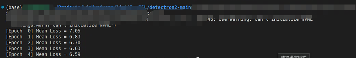
checkpointer.save("my_model")笔者标注:到这一步,就可以进行训练,5个epoch案例
保存的model如下
![]()
Finetuning with Detectron2
笔者标注:到这一步,利用上述训练后的权重训练任何一个Detectron2 脚本
现在,任何 Detectron2 脚本都可以使用上述权重。例如,您可以使用 Detectron2 工具中的 train_net.py 脚本:
笔者标注:使用tool文件夹中的 train_net.py ,注意别找错了

python train_net.py --config-file ../configs/COCO-InstanceSegmentation/mask_rcnn_R_50_FPN_1x.yaml \
    MODEL.WEIGHTS path/to/my_model.pth \
    MODEL.PIXEL_MEAN 123.675,116.280,103.530 \
    MODEL.PIXEL_STD 58.395,57.120,57.375 \
    INPUT.FORMAT RGB
笔者标注:若是用不习惯上述代码,找到mask_rcnn_R_50_FPN_1x.yaml

笔者标注:找到上面的文件后把参数改成下面这样
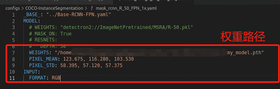
笔者标注:其他文件的修改可以参考该博客:detectron2:使用tools/train_net.py脚本命令行参数训练自己coco格式的数据集_file "tools/train_net.py", line 22, in <module> fr-CSDN博客
SimCLRTransform 默认会对输入图像进行 ImageNet 归一化处理。因此,我们也必须在训练时对输入图像进行归一化处理。由于 Detectron2 使用的输入空间范围为 0 - 255,因此我们使用上述数字。
注释:由于模型是使用 RGB 输入格式的图像预先训练的,因此有必要如上述所示设置像素平均值和像素标准值的排列顺序。