一、方法简述
在Kmeans算法中最终聚类数量K的选择主要通过两个方法综合判断:
-
Elbow Method
这是一种绘制k值范围的平方和的方法。如果此图看起来像一只手臂,则k是选择的类似肘部的值。从这个肘值开始,平方和(惯性)开始以线性方式减小,因此被认为是最佳值。
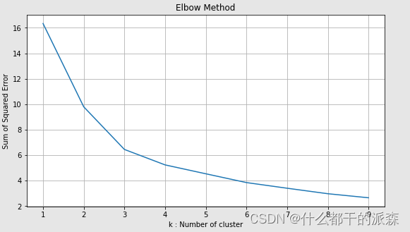
上图的最佳K值为3 -
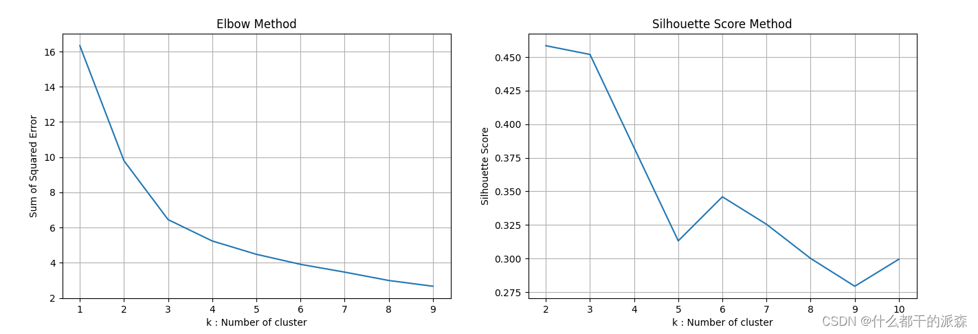
Silhouette Score Method
这是一种根据数据点与彼此相似的其他数据点的聚类程度来评估聚类质量的方法。使用距离公式计算该分数,并且选择具有最高分数的k值用于建模。
具体来说,Silhouette Score 是一种衡量聚类结果质量的指标,它结合了聚类内部的紧密度和不同簇之间的分离度。对于每个数据点,Silhouette Score 考虑了以下几个因素:
1.紧密度:数据点到同簇其他点的平均距离
2.分离度:数据点到最近不同簇的平均距离
设紧密度为a,分离度为b,Silhouette Score 计算公式为 ( b − a ) / m a x ( a , b ) (b - a) / max(a, b) (b−a)/max(a,b)。该值的范围在 -1 到 1 之间,越接近 1 表示数据点聚类得越好,越接近 -1 则表示聚类结果较差。

上图的最佳值为2,3,4
综合两种方法进行判断后,K值选3较为合适
二、使用到的数据集
- 用到的数据集:
各国发展水平统计信息↓
https://download.csdn.net/download/weixin_43721000/88480791 - 字段解释:
country : 国名
child_mort : 每1000个婴儿的5年死亡率
exports : 人均商品和服务出口,以人均国内生产总值的百分比给出
health : 人均卫生支出总额,以人均国内生产总值的百分比给出
imports : 人均商品和服务进口,以人均国内生产总值的百分比给出
Income : 人均净收入
Inflation : 国内生产总值年增长率的测算(通货膨胀率)
life_expec : 如果按照目前的死亡率模式,新生儿的平均寿命是多少年
total_fer : 如果目前的年龄生育率保持不变,每个妇女生育的孩子数量
gdpp : 人均国内生产总值,计算方法是国内生产总值除以总人口 - 任务类型:
对所有国家发展水平聚类,确定待援助国家,涵盖算法:K-Means、DBSCAN、Hierarchical
三、代码实现
import pandas as pd
import matplotlib.pyplot as plt
import seaborn as sns
pd.options.display.float_format = '{:.2f}'.format
import warnings
warnings.filterwarnings('ignore')

from sklearn.cluster import KMeans
from sklearn.metrics import silhouette_score
from sklearn.preprocessing import MinMaxScaler, StandardScaler


def show_elbow_and_silhouette_score(data_values):
    '''
    1.计算Elbow Method
    2.计算Silhouette Score Method
    3.绘图
    :return:
    '''
    sse = {

    }
    sil = []
    kmax = 10
    fig = plt.subplots(nrows=1, ncols=2, figsize=(20, 5))

    # Elbow Method :
    plt.subplot(1, 2, 1)
    for k in range(1, 10):
        kmeans = KMeans(n_clusters=k, max_iter=1000).fit(data_values)
        sse[k] = kmeans.inertia_  # Inertia: Sum of distances of samples to their closest cluster center
    sns.lineplot(x=list(sse.keys()), y=list(sse.values()))
    plt.title('Elbow Method')
    plt.xlabel("k : Number of cluster")
    plt.ylabel("Sum of Squared Error")
    plt.grid()

    # Silhouette Score Method
    plt.subplot(1, 2, 2)
    for k in range(2, kmax + 1):
        kmeans = KMeans(n_clusters=k).fit(data_values)
        labels = kmeans.labels_
        sil.append(silhouette_score(data_values, labels, metric='euclidean'))
    sns.lineplot(x=range(2, kmax + 1), y=sil)
    plt.title('Silhouette Score Method')
    plt.xlabel("k : Number of cluster")
    plt.ylabel("Silhouette Score")
    plt.grid()

    plt.show()


if __name__ == '__main__':


    # 读取数据
    data = pd.read_csv('./data/Country-data.csv')
    print(data.head())
    #                country  child_mort  exports  ...  life_expec  total_fer   gdpp
    # 0          Afghanistan       90.20    10.00  ...       56.20       5.82    553
    # 1              Albania       16.60    28.00  ...       76.30       1.65   4090
    # 2              Algeria       27.30    38.40  ...       76.50       2.89   4460
    # 3               Angola      119.00    62.30  ...       60.10       6.16   3530
    # 4  Antigua and Barbuda       10.30    45.50  ...       76.80       2.13  12200


    # 数据降维
    # 将较为细分的领域数据合并
    # health <== child_mort, health, life_expec, total_fer
    # trade <== imports, exports
    # finance <== income, inflation, gdpp
    # 最终由9个维度降至3维
    df = pd.DataFrame()
    df['Health'] = (data['child_mort'] / data['child_mort'].mean()) + (data['health'] / data['health'].mean()) + (
                data['life_expec'] / data['life_expec'].mean()) + (data['total_fer'] / data['total_fer'].mean())
    df['Trade'] = (data['imports'] / data['imports'].mean()) + (data['exports'] / data['exports'].mean())
    df['Finance'] = (data['income'] / data['income'].mean()) + (data['inflation'] / data['inflation'].mean()) + (
                data['gdpp'] / data['gdpp'].mean())
    print(df.head())
    #    Health  Trade  Finance
    # 0    6.24   1.20     1.35
    # 1    3.04   1.72     1.47
    # 2    3.39   1.60     3.17
    # 3    6.47   2.43     3.49
    # 4    2.96   2.36     2.24


    # 数据归一化
    mms = MinMaxScaler()  # Normalization
    # ss = StandardScaler()  # Standardization
    df['Health'] = mms.fit_transform(df[['Health']])
    df['Trade'] = mms.fit_transform(df[['Trade']])
    df['Finance'] = mms.fit_transform(df[['Finance']])
    df.insert(loc=0, value=list(data['country']), column='Country')
    print(df.head())
    #                Country  Health  Trade  Finance
    # 0          Afghanistan    0.63   0.14     0.08
    # 1              Albania    0.13   0.20     0.09
    # 2              Algeria    0.18   0.19     0.21
    # 3               Angola    0.66   0.28     0.24
    # 4  Antigua and Barbuda    0.12   0.28     0.15


    # 取出归一化之后的各项特征张量
    data_values = df.drop(columns=['Country']).values  # Feature Combination : Health - Trade - Finance
    print(data_values)
    # [[0.6257404  0.13961443 0.07981958]
    #  [0.12745148 0.19990106 0.08875623]
    #  [0.18248518 0.18662177 0.2128085 ]
    #  [0.66138147 0.28305774 0.23694587]
    #      ...       ...        ...
    #  [0.17006974 0.40338563 0.12143593]
    #  [0.39745068 0.17024776 0.22963179]
    #  [0.52690852 0.18140481 0.13499709]]


    # 聚类并绘制 elbow 和 silhouette_score 方法的图像
    show_elbow_and_silhouette_score(data_values)
四、结论
- Elbow Method 显示肘部位置 K=3
- Silhouette Score Method 显示的较高分数在 K=2,3 时表现较好
- 综合两个方法最终确认 K的选值为 3