python——pandas的时间序列分析详解

一、时间序列

1.1 时间序列

1.2 创建时间序列

一、时间序列

1.1 时间序列

时间序列是指多个时间点上形成的数值序列，它既可以是定期的，也可以是不定期出现的。

时间序列的数据主要有以下几种：

时间戳：timestamp：表示特定的某个时刻，比如现在。
时期：period：比如2022年或者2022年3月。
时间间隔：interval：由起始时间戳和结束时间戳表示。

1.2 创建时间序列

在Pandas中，最基本的时间序列类型就是以时间戳为索引的Series对象。

时间戳使用Timestamp（Series派生的子类）对象表示，该对象与datetime具有高度的兼容性，可以直接通过to_datetime()函数将datetime转换为TimeStamp对象。

例如：

import pandas as pd
from datetime import datetime
import numpy as np

print(pd.to_datetime('20200828142123'))      # 将datetime转换为Timestamp对象，年月日 时秒分

当传入的是多个datetime组成的列表，则Pandas会将其强制转换为DatetimeIndex类对象。

# 传入多个datetime字符串
date_index = pd.to_datetime(['20200820151423', '20200828212325', '20200908152360'])
print(date_index)
按照索引获取时间戳：

for i in range(len(date_index)):
    print(date_index[i])

pandas时间戳为索引的Series对象

# 创建时间序列类型的Series对象
date_index = pd.to_datetime(['20200820151423', '20200828212325', '20200908152360'])
# 创建以时间戳为索引的series对象
date_ser = pd.Series([11, 22, 33], index=date_index)
print(date_ser)

也可将包含多个datetime对象的列表传给index参数，同样能创建具有时间戳索引的Series对象。

# 指定索引为多个datetime的列表
date_list = [datetime(2020, 1, 1), datetime(2020, 1, 15),
             datetime(2020, 2, 20), datetime(2020, 4, 1),
             datetime(2020, 5, 5), datetime(2020, 6, 1)]
time_se = pd.Series(np.arange(6), index=date_list)
print(time_se)

DataFrame对象具有时间戳索引

data_demo = [[11, 22, 33], [44, 55, 66],
             [77, 88, 99], [12, 23, 34]]
date_list = [datetime(2020, 1, 23), datetime(2020, 2, 15),
             datetime(2020, 5, 22), datetime(2020, 3, 30)]
time_df = pd.DataFrame(data_demo, index=date_list)
print(time_df)

1.3 通过时间戳索引选取子集

# 指定索引为多个日期字符串的列表,要有相同的格式
date_list = ['2017.05.30', '2019.02.01',
             '2017.6.1', '2018.4.1',
             '2019.6.1', '2020.1.23']
# 将日期字符串转换为DatetimeIndex
date_index = pd.to_datetime(date_list)
# 创建以DatetimeIndex 为索引的Series对象
date_se = pd.Series(np.arange(6), index=date_index)
print(date_se)

选取子集：

1、通过位置索引获取子集数据

print(date_se[3])

2、使用datetime构造的日期获取数据

#根据datetime构造日期获取
date_time = datetime(2018,4,1)
print(date_se[date_time])

3、通过符合格式要求的日期字符串获取

#传入相应的符合日期的字符串获取
print(date_se['20180401'])
print(date_se['2018.04.01'])
print(date_se['2018/04/01'])
print(date_se['2018-04-01'])
print(date_se['04/01/2018'])

4、直接用指定的年份或者月份操作索引来获取某年的数据

print(date_se['2017'])

5、使用过truncate()方法截取 Series或DataFrame对象

truncate(before = None,after = None,axis = None,copy = True)

before – 表示截断此索引值之前的所有行。
after – 表示截断此索引值之后的所有行。
axis – 表示截断的轴，默认为行索引方向。

# 扔掉2018-1-1之前的数据
sorted_se = date_se.sort_index()
print(sorted_se.truncate(before='2018-1-1'))

# 扔掉2018-7-31之后的数据
print(sorted_se.truncate(after='2018-7-31'))

二、固定频率的时间序列

2.1 固定频率时间序列的创建

Pandas中所提供的date_range()函数，主要用于生成一个具有固定频率的DatetimeIndex对象。

参数说明：

start：表示起始日期，默认为None。
end：表示终止日期，默认为None。
periods：表示产生多少个时间戳索引值。
freq：用来指定计时单位。

注意：

start、end、periods、freq这四个参数至少要指定三个参数，否则会出现错误。

用法如下：

1.当调用date_range()函数创建DatetimeIndex对象时，如果只是传入了开始日期（start参数）与结束日期（end参数），则默认生成的时间戳是按天计算的，即freq参数为D

# 创建DatetimeIndex对象时，只传入开始日期与结束日期
print(pd.date_range('2020/08/10', '2023/08/20'))

2.若只是传入了开始日期或结束日期，则还需要用periods参数指定产生多少个时间戳。

# 创建DatetimeIndex对象时，传入start与periods参数
print(pd.date_range(start='2020/08/10', periods=5))

# 创建DatetimeIndex对象时，传入end与periods参数，往前推
print(pd.date_range(end='2020/08/10', periods=5))

3.如果希望时间序列中的时间戳都是每周固定的星期日，则可以在创建DatetimeIndex时将freq参数设为“W-SUN”。

dates_index = pd.date_range('2020-01-01',         # 起始日期
                            periods=5,            # 周期
                            freq='W-SUN')         # 频率
print(dates_index)

4.如果日期中带有与时间相关的信息，且想产生一组被规范化到当天午夜的时间戳，可以将normalize参数的值设为True。

# 创建DatetimeIndex，并指定开始日期、产生日期个数、默认的频率，以及时区
date_index = pd.date_range(start='2020/8/1 12:13:30', periods=5,
              tz='Asia/Hong_Kong')
print(date_index)

#规范化时间戳
date_index2 = pd.date_range(start='2020/8/1 12:13:30', periods=5,
              normalize=True, tz='Asia/Hong_Kong')
print(date_index2)

2.2 时间序列的频率和偏移量

1.默认生成的时间序列数据是按天计算的，即频率为“D”。

“D”是一个基础频率，通过用一个字符串的别名表示，比如“D”是“day”的别名。
频率是由一个基础频率和一个乘数组成的，比如，“5D”表示每5天。

其他频率说明如下：

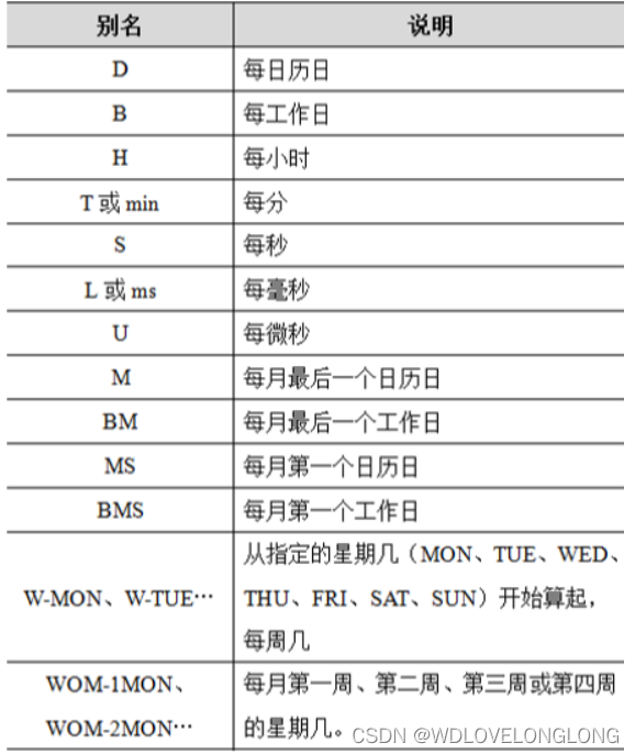
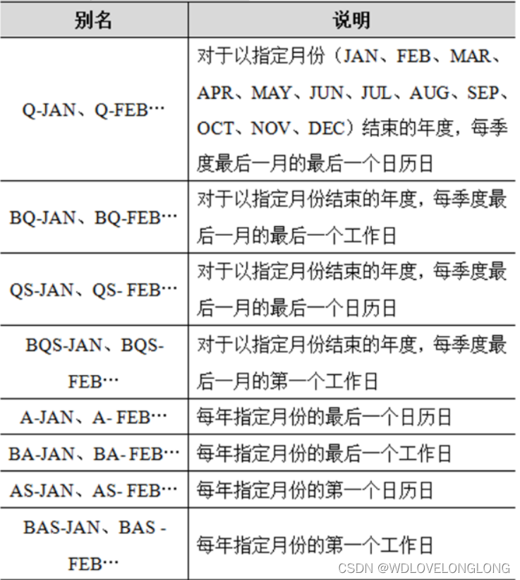
用于指定freq属性：

date_time5D = pd.date_range(start='2020/2/1', end='2020/2/28', freq='5D')
print(date_time5D)

2.每个基础频率还可以跟着一个被称为日期偏移量的DateOffset对象。如果想要创建一个DateOffset对象，则需要先导入pd.tseries.offsets模块后才行。

可以指定偏移量创建时间序列,同时，创建14天10小时的偏移量，可以换算为两周零十个小时，其中“周”使用Week类型表示的，“小时”使用Hour类型表示，它们之间可以使用加号连接。

import pandas as pd
from datetime import datetime
import numpy as np
from pandas.tseries.offsets import *

date_offset1 = DateOffset(weekday=2,hour=10)
'''            - year
            - month
            - day
            - weekday
            - hour
            - minute
            - second
            - microsecond
            - nanosecond.'''
date_offset2 = Week(2) + Hour(10)

date_index1 = pd.date_range('2020/3/1',periods=5,freq=date_offset1)
date_index2 = pd.date_range('2020/3/1',periods=5,freq=date_offset2)
print(date_index1)
print(date_index2)

2.3 时间序列的移动

移动是指沿着时间轴方向将数据进行前移或后移。如下图所示：

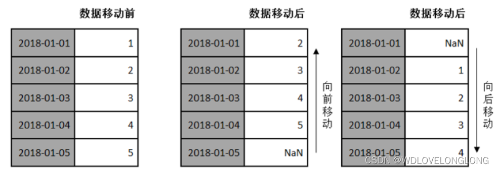
Pandas对象中提供了一个shift()方法，用来前移或后移数据，但数据索引保持不变。

用法如下：

shift(periods=1, freq=None, axis=0)
#periods – 表示移动的幅度，可以为正数，也可以为负数，默认值是1，代表移动一次。
date_index = pd.date_range('2020/01/01', periods=5)
time_ser = pd.Series(np.arange(5) + 1, index=date_index)
print(time_ser)
# 向后移动一次
print(time_ser.shift(1))
#向前移动一次
print(time_ser.shift(-1))

三、时间周期及计算

3.1 时间周期的创建

1.Period类表示一个标准的时间段或时期，比如某年、某月、某日、某小时等。

创建Period类对象的方式比较简单，只需要在构造方法中以字符串或整数的形式传入一个日期即可。

# 创建Period对象，表示从2020-01-01到2020-12-31之间的时间段
period = pd.Period(2020)
print(period)

# 表示从2019-06-01到2019-06-30之间的整月时间
period = pd.Period('2019/6')
print(period)

2.Period对象能够参与数学运算。

如果Period对象加上或者减去一个整数，则会根据具体的时间单位进行位移操作。

period = period + 1   # Period对象加上一个整数
print(period)

如果具有相同频率的两个Period对象进行数学运算，那么计算结果为它们的单位数量。

# 表示从2019-06-01到2019-06-30之间的整月时间
period = pd.Period('2019/6')
print(period)

period = period + 1   # Period对象加上一个整数
print(period)

# 创建一个与period频率相同的时期
other_period = pd.Period(201401, freq='M' )
print(period - other_period)

3.如果希望创建多个Period对象，且它们是固定出现的，则可以通过period_range()函数实现。

返回一个PeriodIndex对象，它是由一组时期对象构成的索引，示例如下：

period_index = pd.period_range('2014.1.8', '2014.5.31', freq='M')
print(period_index)

4.除了使用上述方式创建PeriodIndex外，还可以直接在PeriodIndex的构造方法中传入一组日期字符串。

period_index = pd.period_range('2014.1.8', '2014.5.31', freq='M')
print(period_index)

str_list = ['2012', '2013', '2014']
period_list = pd.PeriodIndex(str_list, freq='A-DEC')
print(period_list)
time_index = pd.Series(np.arange(len(period_index)) + 1,index = period_index)
print(time_index)

注意：DatetimeIndex是用来指代一系列时间点的一种索引结构，而PeriodIndex则是用来指代一系列时间段的索引结构。

3.2 时期的频率转化

1.Pandas中提供了一个asfreq()方法来转换时期的频率。

asfreq（freq，method = None，how = None，normalize = False，fill_value = None ）

参数说明：

freq – 表示计时单位。
how – 可以取值为start或end，默认为end。
normalize – 表示是否将时间索引重置为午夜。
fill_value – 用于填充缺失值的值。

# 创建时期对象
period = pd.Period('2019', freq='A-DEC')
print(period)
period_freq_start = period.asfreq('M', how='start')
print(period_freq_start)
period_freq_end = period.asfreq('M',how='end')
print(period_freq_end)

四、重采样

4.1 重采样方法（resample）

1.Pandas中的resample()是一个对常规时间序列数据重新采样和频率转换的便捷的方法。

resample(rule, how=None, axis=0, fill_method=N

date_index = pd.date_range('2019.7.8', periods=30)
time_ser = pd.Series(np.arange(len(date_index)) + 1, index=date_index)
print(time_ser)

print(time_ser.resample('W-MON').mean())

one, closed=None, label=None, ...)

参数说明：

rule – 表示重采样频率的字符串或DateOffset。
fill_method – 表示升采样时如何插值。
closed – 设置降采样哪一端是闭合的。

1.通过resample()方法对数据重新采样

注意：how参数不再建议使用，而是采用新的方式“.resample(…).mean()”求平均值。

2.如果重采样时传入closed参数为left，则表示采样的范围是左闭右开型的。

即位于某范围的时间序列中，开头的时间戳包含在内，结尾的时间戳是不包含在内的。

print(time_ser.resample('W-MON', closed='left').mean())

4.2 降采样

1.降采样时间颗粒会变大，数据量是减少的。为了避免有些时间戳对应的数据闲置，可以利用内置方法聚合数据。

例如股票数据比较常见的是OHLC重采样，包括开盘价、最高价、最低价和收盘价。

Pandas中专门提供了一个ohlc()方法。

date_index = pd.date_range('2020/06/01', periods=30)
shares_data = np.random.rand(30)
time_ser = pd.Series(shares_data, index=date_index)
print(time_ser)
result = time_ser.resample('7D').ohlc()        # OHLC重采样 得到七天中的开盘价，最高价，最低价以及收盘价
print(result)

2.降采样相当于另外一种形式的分组操作，它会按照日期将时间序列进行分组，之后对每个分组应用聚合方法得出一个结果。

# 通过groupby技术实现降采样
result = time_ser.groupby(lambda x: x.week).mean()
print(result)

4.3 升采样

1.升采样的时间颗粒是变小的，数据量会增多，这很有可能导致某些时间戳没有相应的数据。

遇到这种情况，常用的解决办法就是插值，具体有如下几种方式：

通过ffill(limit)或bfill(limit)方法，取空值前面或后面的值填充，limit可以限制填充的个数。
通过fillna(‘ffill’)或fillna(‘bfill’)进行填充，传入ffill则表示用NaN前面的值填充，传入bfill则表示用后面的值填充。
通过使用interpolate()方法根据插值算法补全数据。

data_demo = np.array([['101', '210', '150'], ['330', '460', '580']])
date_index = pd.date_range('2020/06/10', periods=len(data_demo), freq='W-SUN')
time_df = pd.DataFrame(data_demo, index=date_index,
columns=['A产品', 'B产品', 'C产品'])
print(time_df)

#增加采样时间，但没有填充数据
time_df_asfreq = time_df.resample('D').asfreq()
print(time_df_asfreq)

#用前面的数据填充
time_df_ffill = time_df.resample('D').ffill()
print(time_df_ffill)

#用后面的数据 填充
time_df_bfill = time_df.resample('D').bfill()
print(time_df_bfill)

五、数据统计——滑动窗口

5.1 滑动窗口

1.滑动窗口指的是根据指定的单位长度来框住时间序列，从而计算框内的统计指标。

相当于一个长度指定的滑块在刻度尺上面滑动，每滑动一个单位即可反馈滑块内的数据。

示例如下：

某分店按天统计了2017年全年的销售数据，现在总经理想抽查分店8月28日（七夕）的销售情况，如果只是单独拎出来当天的数据，则这个数据比较绝对，无法很好地反映出这个日期前后销售的整体情况。

为了提升数据的准确性，可以将某个点的取值扩大到包含这个点的一段区间，用区间内的数据进行判断。

可以将8月24日到9月2日的数据拿出来，求此区间的平均值作为抽查结果。

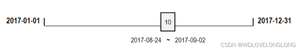
这个区间就是窗口，它的单位长度为10，数据是按天统计的，所以统计的是10天的平均指标，这样显得更加合理，可以很好地反映了七夕活动的整体情况。

3.移动窗口就是窗口向一端滑行，每次滑行并不是区间整块的滑行，而是一个单位一个单位的滑行。

例如，窗口向右边滑行一个单位，此时窗口框住的时间区间范围为2017-08-25到2017-09-03。

每次窗口移动，一次只会移动一个单位的长度，并且窗口的长度始终为10个单位长度，直至移动到末端。

由此可知，通过滑动窗口统计的指标会更加平稳一些，数据上下浮动的范围会比较小。

5.2 滑动窗口法

Pandas中提供了一个窗口方法rolling()。

rolling(window, min_periods=None, center=False, win_type=None, on=None, axis=0, closed=None)

参数说明：

window – 表示窗口的大小。
min_periods – 每个窗口最少包含的观测值数量。
center – 是否把窗口的标签设置为居中。
win_type – 表示窗口的类型。
closed – 用于定义区间的开闭。

year_data = np.random.randn(365)
date_index = pd.date_range('2017-01-01', '2017-12-31', freq='D')
ser = pd.Series(year_data, date_index)
print(ser.head()) #打印前几个数据 默认为5

#画图观察
import matplotlib.pyplot as plt

ser.plot(style='y--')
ser_window = ser.rolling(window=10).mean()
ser_window.plot(style='b')
plt.show()