-------往期目录------
天鹰优化器
Aquila Optimizer(AO),灵感来自Aquila在捕捉猎物过程中的自然界行为。因此,所提出的AO算法的优化过程分为四种方法:用垂直弯腰的高腾空选择搜索空间,用轮廓飞行和短滑翔攻击在发散搜索空间内探索,用低飞行和慢下降攻击在收敛搜索空间内利用,以及用步行和抓取猎物俯冲。为了验证新的优化器为不同优化问题找到最优解的能力,进行了一系列实验。
提示:以下是本篇文章正文内容,下面案例可供参考
一、第一种搜索方法
Aquila识别猎物区域,并通过垂直弯腰的高飞选择最佳狩猎区域。在这里,天鹰从高飞广泛探索者来确定170°搜索空间的区域,猎物在哪里。图1显示了Aquila高飞垂直弯腰的行为。这种行为在数学上表现为下列等式。
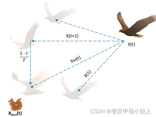
图1:Aquila高飞垂直弯腰的行为
X 1 ( t + 1 ) = X b e s t ( t ) × ( 1 − t T ) + ( X M ( t ) − X b e s t ( t ) ∗ r a n d ) X_{1}(t+1)=X_{b e s t}(t)\times\left(1-{\frac{t}{T}}\right)+(X_{M}(t)-X_{b e s t}(t)*r a n d) X1(t+1)=Xbest(t)×(1−Tt)+(XM(t)−Xbest(t)∗rand)
X M ( t ) = 1 N ∑ i = 1 N X i ( t ) , ∀ j = 1 , 2 , . . . , D i m X_{M}(t)={\frac{1}{N}}\sum_{i=1}^{N}X_{i}(t),\forall j=1,2,...,D i m XM(t)=N1i=1∑NXi(t),∀j=1,2,...,Dim
其中, X 1 ( t + 1 ) X_{1}(t+1) X1(t+1)是t的下一次迭代的解,由第一种搜索方法( X 1 X_{1} X1)生成。 X b e s t ( t ) X_{b e s t}(t) Xbest(t)是直到第t次迭代的最佳获得解,这反映了猎物的近似位置。这个方程 1 − t T 1-{\frac{t}{T}} 1−Tt用于控制通过迭代的扩展搜索(探索)。 X M ( t ) X_M(t) XM(t)表示在第t次迭代时连接的当前解的位置平均值, r a n d ∈ [ 0 , 1 ] rand∈[0,1] rand∈[0,1].
二、第二种搜素方法
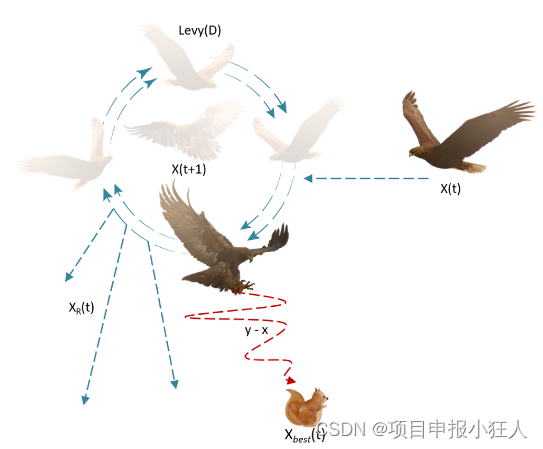
X 2 ( t + 1 ) = X b e s t ( t ) × L e v y ( D ) + X R ( t ) + ( y − x ) ∗ r a n d , X_{2}(t+1)=X_{b e s t}(t)\times L e v y(D)+X_{R}(t)+(y-x)*r a n d, X2(t+1)=Xbest(t)×Levy(D)+XR(t)+(y−x)∗rand,
其中 X 2 ( t + 1 ) X_2(t+1) X2(t+1)是 t t t 的下一次迭代的解,由第二种搜索方法 X 2 X_2 X2生成, D D D是维数空间, L e v y ( D ) Levy(D) Levy(D)是 l e v y levy levy飞行分布函数,使用公式计算, X R ( t ) X_R(t) XR(t)是第 t t t 次迭代时在 [ 1 , N ] [1,N] [1,N]范围内取的随机解.
L e v y ( D ) = s × u × σ ∣ v ∣ 1 β L e v y(D)=s\times{\frac{u\times\sigma}{|v|^{\frac{1}{β}}}} Levy(D)=s×∣v∣β1u×σ
其中s是固定为0.01的常量值, u u u和 v v v 是 0 0 0到1之间的随机数, σ σ σ 使用下列等式计算:
σ = Γ ( 1 + β ) × sin ( π β 2 ) Γ ( 1 + β 2 ) × β × 2 β − 1 2 \sigma={\frac{\Gamma(1+\beta)\times\sin\left({\frac{\pi\beta}{2}}\right)}{\Gamma\left({\frac{1+\beta}{2}}\right)\times\beta\times2^{\frac{\beta-1}{2}}}} σ=Γ(21+β)×β×22β−1Γ(1+β)×sin(2πβ)
其中β是固定为1.5的常数值.
r = r 1 + U × D 1 θ = − ω × D 1 + θ 1 θ 1 = 3 × π 2 \begin{array}{c}{
{r=r_{1}+U\times D_{1}}}\\ {
{}}\\ {
{\theta=-\omega\times D_{1}+\theta_{1}}}\\ {
{}}\\ {
{\theta_{1}=\frac{3\times\pi}{2}}}\end{array} r=r1+U×D1θ=−ω×D1+θ1θ1=23×π
R 1 ∈ [ 1 , 20 ] R_1∈[1,20] R1∈[1,20],用于固定搜索周期数, U U U是一个固定为0.00565的小值。 D 1 D_1 D1是从1到搜索空间长度(Dim)的整数, ω \omega ω是一个固定为0.005的小值。以螺旋形状显示了AO的行为
x = r × s i n ( θ ) y = r × cos ( θ ) r = − 0.005 × D 1 + 3 × π 2 \begin{array}{c}{
{x=r\times s\mathrm{in}(\theta)}}\\ {
{y=r\times\cos(\theta)}}\\ {
{r=-0.005\times D_{1}+\frac{3\times\pi}{2}}}\end{array} x=r×sin(θ)y=r×cos(θ)r=−0.005×D1+23×π
三、第三种搜素方法
在第三种方法(X3)中,当准确指定猎物区域,并且天鹰准备着陆和攻击时,天鹰垂直下降,进行初步攻击以发现猎物反应。
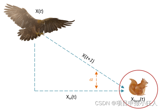
称为慢速下降攻击的低空飞行。在这里,AO利用目标的选定区域接近猎物并进行攻击。图显示了Aquila低空飞行慢速下降攻击的行为
X 3 ( t + 1 ) = ( X b e s t ( t ) − X M ( t ) ) × α − r a n d + ( ( U B − L B ) × r a n d + L B ) × δ X_{3}(t+1)=(X_{b e s t}(t)-X_{M}(t))\times\alpha-r a n d+((U B-L B)\times r a n d+L B)\times\delta X3(t+1)=(Xbest(t)−XM(t))×α−rand+((UB−LB)×rand+LB)×δ
X 3 ( t + 1 ) X_3(t+1) X3(t+1)是由第三种搜索方法 X 3 X_3 X3生成的t的下一次迭代的解。 X B e s t ( t ) X_Best(t) XBest(t)是指第i次迭代前猎物的近似位置(最佳获得的解), X M ( t ) X_M(t) XM(t)是第t次迭代时当前解的平均值,使用等式计算。rand是0到1之间的随机值。 α \alpha α和 δ \delta δ是本文固定为小值(0.1)的开发调整参数。 L B L_B LB表示给定问题的下界, U B U_B UB表示200的上界.
四、第四种搜索方法
接近猎物时,Aquila根据猎物的随机运动在陆地上攻击猎物。这种方法称为步行并抓住猎物。这里,最后,AO在最后一个位置攻击猎物。图显示了Aquila步行并抓住猎物的行为。
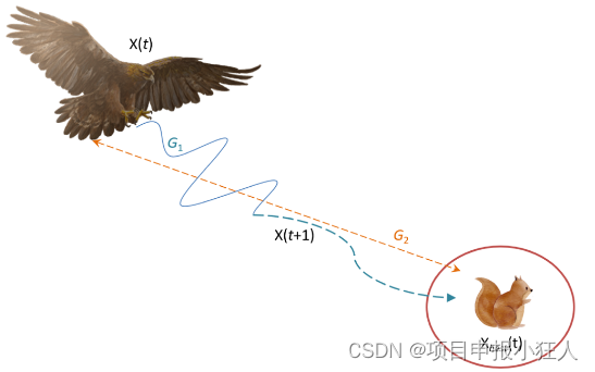
X 4 ( t + 1 ) = Q F × X b e x ( t ) − ( G 1 × X ( t ) × r a n d ) − G 2 × L e ν y ( D ) + r a n d × G 1 \begin{array}{c}{
{X_{4}(t+1)=Q F\times X_{b e x}(t)-(G_{1}\times X(t)\times r a n d)-G_{2}\times L e\nu y(D)+r a n d×G_1}}\\{
{}}\end{array} X4(t+1)=QF×Xbex(t)−(G1×X(t)×rand)−G2×Leνy(D)+rand×G1
Q F ( t ) = t r a n d − 1 ( 1 − T ) 2 Q F(t)=t^{\frac{rand-1}{(1-T)^{2}}} QF(t)=t(1−T)2rand−1
G 1 = 2 × r a n d − 1 G 2 = 2 × ( 1 − t T ) \begin{array}{c}{
{G_{1}=2\times r a n d-1}}\\ {
{}}\\ {
{G_{2}=2\times\left(1-\frac{t}{T}\right)}}\end{array} G1=2×rand−1G2=2×(1−Tt)
Q F ( t ) QF(t) QF(t)是第 i t h i^{th} ith次迭代时的质量函数值, r a n d rand rand是0到1之间的随机值。t和T分别表示当前迭代和最大迭代次数。 L e v y ( D ) Levy(D) Levy(D)是使用方程计算的 l e v y levy levy飞行分布函数
代码实现
完整代码请私信领取:
function [Best_FF,Best_P,conv]=AO(N,T,LB,UB,Dim,F_obj)
Best_P=zeros(1,Dim);
Best_FF=inf;


X=initialization(N,Dim,UB,LB);
Xnew=X;
Ffun=zeros(1,size(X,1));
Ffun_new=zeros(1,size(Xnew,1));

t=1;


alpha=0.1;
delta=0.1;

while t<T+1
    for i=1:size(X,1)
        F_UB=X(i,:)>UB;
        F_LB=X(i,:)<LB;
        X(i,:)=(X(i,:).*(~(F_UB+F_LB)))+UB.*F_UB+LB.*F_LB;
        Ffun(1,i)=F_obj(X(i,:));
        if Ffun(1,i)<Best_FF
            Best_FF=Ffun(1,i);
            Best_P=X(i,:);
        end
    end


    G2=2*rand()-1; % Eq. (16)
    G1=2*(1-(t/T));  % Eq. (17)
    to = 1:Dim;
    u = .0265;
    r0 = 10;
    r = r0 +u*to;
    omega = .005;
    phi0 = 3*pi/2;
    phi = -omega*to+phi0;
    x = r .* sin(phi);  % Eq. (9)
    y = r .* cos(phi); % Eq. (10)
    QF=t^((2*rand()-1)/(1-T)^2); % Eq. (15)
        %-------------------------------------------------------------------------------------
    for i=1:size(X,1)
        %-------------------------------------------------------------------------------------
        if t<=(2/3)*T
            if rand <0.5
                Xnew(i,:)=Best_P(1,:)*(1-t/T)+(mean(X(i,:))-Best_P(1,:))*rand(); % Eq. (3) and Eq. (4)
                Ffun_new(1,i)=F_obj(Xnew(i,:));
                if Ffun_new(1,i)<Ffun(1,i)
                    X(i,:)=Xnew(i,:);
                    Ffun(1,i)=Ffun_new(1,i);
                end
            else
                %-------------------------------------------------------------------------------------
                Xnew(i,:)=Best_P(1,:).*Levy(Dim)+X((floor(N*rand()+1)),:)+(y-x)*rand;       % Eq. (5)
                Ffun_new(1,i)=F_obj(Xnew(i,:));
                if Ffun_new(1,i)<Ffun(1,i)
                    X(i,:)=Xnew(i,:);
                    Ffun(1,i)=Ffun_new(1,i);
                end
            end
            %-------------------------------------------------------------------------------------
        else
            if rand<0.5
                Xnew(i,:)=(Best_P(1,:)-mean(X))*alpha-rand+((UB-LB)*rand+LB)*delta;   % Eq. (13)
                Ffun_new(1,i)=F_obj(Xnew(i,:));
                if Ffun_new(1,i)<Ffun(1,i)
                    X(i,:)=Xnew(i,:);
                    Ffun(1,i)=Ffun_new(1,i);
                end
            else
                %-------------------------------------------------------------------------------------
                Xnew(i,:)=QF*Best_P(1,:)-(G2*X(i,:)*rand)-G1.*Levy(Dim)+rand*G2; % Eq. (14)
                Ffun_new(1,i)=F_obj(Xnew(i,:));
                if Ffun_new(1,i)<Ffun(1,i)
                    X(i,:)=Xnew(i,:);
                    Ffun(1,i)=Ffun_new(1,i);
                end
            end
        end
    end
    %-------------------------------------------------------------------------------------
    if mod(t,100)==0
        display(['At iteration ', num2str(t), ' the best solution fitness is ', num2str(Best_FF)]);
    end
    conv(t)=Best_FF;
    t=t+1;
end

end
function o=Levy(d)
	beta=1.5;
	sigma=(gamma(1+beta)*sin(pi*beta/2)/(gamma((1+beta)/2)*beta*2^((beta-1)/2)))^(1/beta);
	u=randn(1,d)*sigma;v=randn(1,d);step=u./abs(v).^(1/beta);
	o=step;
end
Abualigah, L., Yousri, D., Elaziz, M.A., Ewees, A.A., A. Al-qaness, M.A., Gandomi, A.H., Aquila Optimizer: A novel meta-heuristic optimization Algorithm, Computers & Industrial Engineering (2021), doi: https://doi.org/10.1016/j.cie.2021.107250