一、数据集
1、目标
知道数据集分为训练集和测试集
会使用sklearn的数据集
2、可用数据集
公司内部,比如百度、微博
数据接口,花钱
政府拥有的数据集
3、在学习阶段用到的数据集
scikit-learn特点:
(1)数据量较小
(2)方便学习
UCI特点:
(1)收录了360个数据集
(2)覆盖科学、生活、经济等领域
(3)数据量几十万
kaggle特点:
(1)大数据竞赛平台
(2)80万科学家
(3)真实数据
(4)数据量巨大
4、网址
kaggle网址:https://www.kaggle.com/datasets
UCI网址:http://archive.ics.uci.edu/ml
scikit-learn网址:http://scikit-learn.org/stable/datasets
5、scikit-learn工具介绍
Machine Learning with Scikit-Learn
(1)python语言的机器学习工具
(2)scikit-learn包含许多知名的机器学习算法的实现
(3)scikit-learn文档完善,容易上手,丰富的API
6、安装scikit-learn
yum install python3 python3-pip
pip3 install -U scikit-learn
pip3 install -U ipython
7、验证安装
$ python3 -m pip show scikit-learn

Name: scikit-learn
Version: 0.24.2
Summary: A set of python modules for machine learning and data mining
Home-page: http://scikit-learn.org
Author: None
Author-email: None
License: new BSD
Location: /usr/local/lib64/python3.6/site-packages
Requires: joblib, scipy, numpy, threadpoolctl

$ python3 -m pip freeze

joblib==1.1.1
numpy==1.19.5
scikit-learn==0.24.2
scipy==1.5.4
threadpoolctl==3.1.0

$ python3 -c "import sklearn; sklearn.show_versions()"

System:
    python: 3.6.8 (default, Jun 20 2023, 11:53:23)  [GCC 4.8.5 20150623 (Red Hat 4.8.5-44)]
executable: /usr/bin/python3
   machine: Linux-3.10.0-1160.92.1.el7.x86_64-x86_64-with-centos-7.9.2009-Core

Python dependencies:
          pip: 9.0.3
   setuptools: 39.2.0
      sklearn: 0.24.2
        numpy: 1.19.5
        scipy: 1.5.4
       Cython: None
       pandas: None
   matplotlib: None
       joblib: 1.1.1
threadpoolctl: 3.1.0

Built with OpenMP: True
8、scikit-learn包含的内容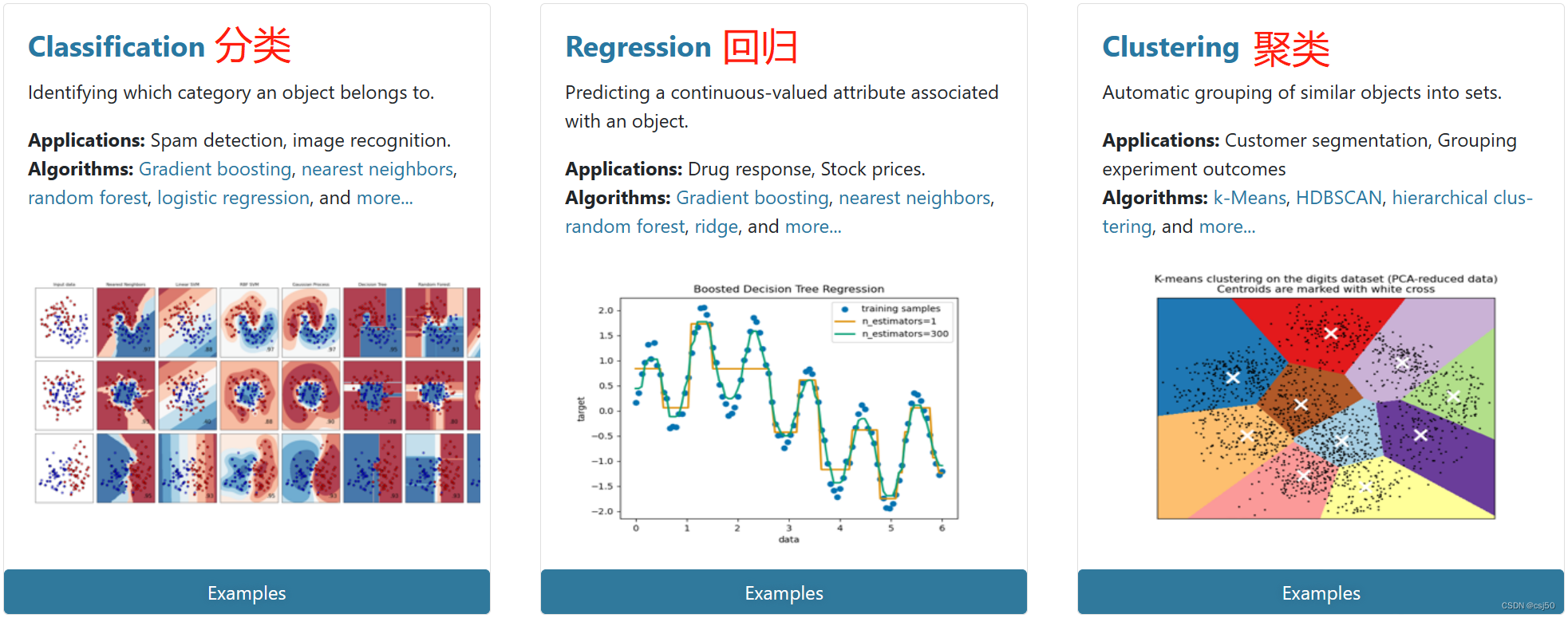

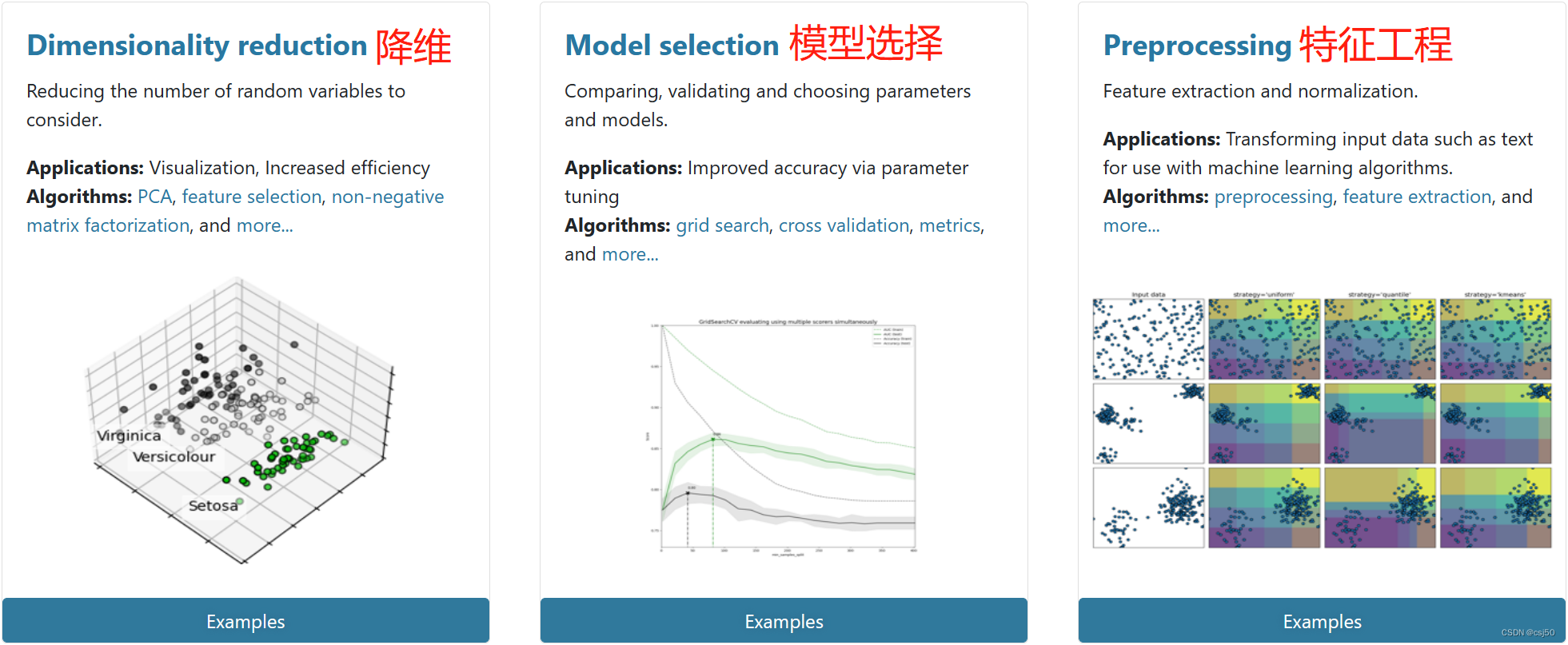
(1)分类、聚类、回归
(2)特征工程
(3)模型选择、调优
二、sklearn数据集
1、scikit-learn数据集API介绍
(1)sklearn.datasets
加载获取流行数据集
datasets.load_*()
获取小规模数据集,数据包含在datasets里
datasets.fetch_*(data_home=None)
获取大规模数据集,需要从网上下载,函数的第一个参数是data_home,表示数据集下载的目录,默认是~/scikit_learn_data/
2、sklearn小数据集
(1)sklearn.datasets.load_iris()
加载并返回鸢尾花数据集
| 名称 | 数量 |
| 类别 | 3 |
| 特征 | 4 |
| 样本数量 | 150 |
| 每个类别数量 | 50 |
(2)sklearn.datasets.load_boston()
加载并返回波士顿房价数据集
| 名称 | 数量 |
| 目标类别 | 5-50 |
| 特征 | 13 |
| 样本数量 | 506 |
3、sklearn大数据集
(1)sklearn.datasets.fetch_20newsgroups(data_home=None,subset='train')
subset:'train'或者'test','all',可选,选择要加载的数据集
训练集的"训练",测试集的"测试",两者的"全部"
4、sklearn数据集的使用
(1)以鸢尾花数据集为例
鸢尾花数据集
特征值--4个:花瓣、花瓣的长度、宽度
目标值--3个:setosa,vericolor,virginica
(2)sklearn数据集返回值介绍
load和fetch返回的数据类型datasets.base.Bunch(字典格式)
data:特征数据数组,是 [n_samples * n_features] 的二维numpy.ndarray数组
target:标签数据,是n_samples的一维numpy.ndarray数组
DESCR:数据描述
feature_names:特证名。新闻数据、手写数字、回归数据集没有
target_names:标签名
(3)建立文件day01_machine_learning.py
from sklearn.datasets import load_iris

def datasets_demo():
    """
    sklearn数据集使用
    """
    #获取数据集
    iris = load_iris()
    print("鸢尾花数据集:\n", iris)
    print("查看数据集描述:\n", iris["DESCR"])
    print("查看特征值的名字:\n", iris.feature_names)
    print("查看特征值几行几列:\n", iris.data.shape)

    return None

if __name__ == "__main__":
    # 代码1:sklearn数据集使用
    datasets_demo()
运行:python3 day01_machine_learning.py
鸢尾花数据集:
 {'data': array([[5.1, 3.5, 1.4, 0.2],
       [4.9, 3. , 1.4, 0.2],
       [4.7, 3.2, 1.3, 0.2],
       [4.6, 3.1, 1.5, 0.2],
       [5. , 3.6, 1.4, 0.2],
       [5.4, 3.9, 1.7, 0.4],
       [4.6, 3.4, 1.4, 0.3],
       [5. , 3.4, 1.5, 0.2],
       [4.4, 2.9, 1.4, 0.2],
       [4.9, 3.1, 1.5, 0.1],
       [5.4, 3.7, 1.5, 0.2],
       [4.8, 3.4, 1.6, 0.2],
       [4.8, 3. , 1.4, 0.1],
       [4.3, 3. , 1.1, 0.1],
       [5.8, 4. , 1.2, 0.2],
       [5.7, 4.4, 1.5, 0.4],
       [5.4, 3.9, 1.3, 0.4],
       [5.1, 3.5, 1.4, 0.3],
       [5.7, 3.8, 1.7, 0.3],
       [5.1, 3.8, 1.5, 0.3],
       [5.4, 3.4, 1.7, 0.2],
       [5.1, 3.7, 1.5, 0.4],
       [4.6, 3.6, 1. , 0.2],
       [5.1, 3.3, 1.7, 0.5],
       [4.8, 3.4, 1.9, 0.2],
       [5. , 3. , 1.6, 0.2],
       [5. , 3.4, 1.6, 0.4],
       [5.2, 3.5, 1.5, 0.2],
       [5.2, 3.4, 1.4, 0.2],
       [4.7, 3.2, 1.6, 0.2],
       [4.8, 3.1, 1.6, 0.2],
       [5.4, 3.4, 1.5, 0.4],
       [5.2, 4.1, 1.5, 0.1],
       [5.5, 4.2, 1.4, 0.2],
       [4.9, 3.1, 1.5, 0.2],
       [5. , 3.2, 1.2, 0.2],
       [5.5, 3.5, 1.3, 0.2],
       [4.9, 3.6, 1.4, 0.1],
       [4.4, 3. , 1.3, 0.2],
       [5.1, 3.4, 1.5, 0.2],
       [5. , 3.5, 1.3, 0.3],
       [4.5, 2.3, 1.3, 0.3],
       [4.4, 3.2, 1.3, 0.2],
       [5. , 3.5, 1.6, 0.6],
       [5.1, 3.8, 1.9, 0.4],
       [4.8, 3. , 1.4, 0.3],
       [5.1, 3.8, 1.6, 0.2],
       [4.6, 3.2, 1.4, 0.2],
       [5.3, 3.7, 1.5, 0.2],
       [5. , 3.3, 1.4, 0.2],
       [7. , 3.2, 4.7, 1.4],
       [6.4, 3.2, 4.5, 1.5],
       [6.9, 3.1, 4.9, 1.5],
       [5.5, 2.3, 4. , 1.3],
       [6.5, 2.8, 4.6, 1.5],
       [5.7, 2.8, 4.5, 1.3],
       [6.3, 3.3, 4.7, 1.6],
       [4.9, 2.4, 3.3, 1. ],
       [6.6, 2.9, 4.6, 1.3],
       [5.2, 2.7, 3.9, 1.4],
       [5. , 2. , 3.5, 1. ],
       [5.9, 3. , 4.2, 1.5],
       [6. , 2.2, 4. , 1. ],
       [6.1, 2.9, 4.7, 1.4],
       [5.6, 2.9, 3.6, 1.3],
       [6.7, 3.1, 4.4, 1.4],
       [5.6, 3. , 4.5, 1.5],
       [5.8, 2.7, 4.1, 1. ],
       [6.2, 2.2, 4.5, 1.5],
       [5.6, 2.5, 3.9, 1.1],
       [5.9, 3.2, 4.8, 1.8],
       [6.1, 2.8, 4. , 1.3],
       [6.3, 2.5, 4.9, 1.5],
       [6.1, 2.8, 4.7, 1.2],
       [6.4, 2.9, 4.3, 1.3],
       [6.6, 3. , 4.4, 1.4],
       [6.8, 2.8, 4.8, 1.4],
       [6.7, 3. , 5. , 1.7],
       [6. , 2.9, 4.5, 1.5],
       [5.7, 2.6, 3.5, 1. ],
       [5.5, 2.4, 3.8, 1.1],
       [5.5, 2.4, 3.7, 1. ],
       [5.8, 2.7, 3.9, 1.2],
       [6. , 2.7, 5.1, 1.6],
       [5.4, 3. , 4.5, 1.5],
       [6. , 3.4, 4.5, 1.6],
       [6.7, 3.1, 4.7, 1.5],
       [6.3, 2.3, 4.4, 1.3],
       [5.6, 3. , 4.1, 1.3],
       [5.5, 2.5, 4. , 1.3],
       [5.5, 2.6, 4.4, 1.2],
       [6.1, 3. , 4.6, 1.4],
       [5.8, 2.6, 4. , 1.2],
       [5. , 2.3, 3.3, 1. ],
       [5.6, 2.7, 4.2, 1.3],
       [5.7, 3. , 4.2, 1.2],
       [5.7, 2.9, 4.2, 1.3],
       [6.2, 2.9, 4.3, 1.3],
       [5.1, 2.5, 3. , 1.1],
       [5.7, 2.8, 4.1, 1.3],
       [6.3, 3.3, 6. , 2.5],
       [5.8, 2.7, 5.1, 1.9],
       [7.1, 3. , 5.9, 2.1],
       [6.3, 2.9, 5.6, 1.8],
       [6.5, 3. , 5.8, 2.2],
       [7.6, 3. , 6.6, 2.1],
       [4.9, 2.5, 4.5, 1.7],
       [7.3, 2.9, 6.3, 1.8],
       [6.7, 2.5, 5.8, 1.8],
       [7.2, 3.6, 6.1, 2.5],
       [6.5, 3.2, 5.1, 2. ],
       [6.4, 2.7, 5.3, 1.9],
       [6.8, 3. , 5.5, 2.1],
       [5.7, 2.5, 5. , 2. ],
       [5.8, 2.8, 5.1, 2.4],
       [6.4, 3.2, 5.3, 2.3],
       [6.5, 3. , 5.5, 1.8],
       [7.7, 3.8, 6.7, 2.2],
       [7.7, 2.6, 6.9, 2.3],
       [6. , 2.2, 5. , 1.5],
       [6.9, 3.2, 5.7, 2.3],
       [5.6, 2.8, 4.9, 2. ],
       [7.7, 2.8, 6.7, 2. ],
       [6.3, 2.7, 4.9, 1.8],
       [6.7, 3.3, 5.7, 2.1],
       [7.2, 3.2, 6. , 1.8],
       [6.2, 2.8, 4.8, 1.8],
       [6.1, 3. , 4.9, 1.8],
       [6.4, 2.8, 5.6, 2.1],
       [7.2, 3. , 5.8, 1.6],
       [7.4, 2.8, 6.1, 1.9],
       [7.9, 3.8, 6.4, 2. ],
       [6.4, 2.8, 5.6, 2.2],
       [6.3, 2.8, 5.1, 1.5],
       [6.1, 2.6, 5.6, 1.4],
       [7.7, 3. , 6.1, 2.3],
       [6.3, 3.4, 5.6, 2.4],
       [6.4, 3.1, 5.5, 1.8],
       [6. , 3. , 4.8, 1.8],
       [6.9, 3.1, 5.4, 2.1],
       [6.7, 3.1, 5.6, 2.4],
       [6.9, 3.1, 5.1, 2.3],
       [5.8, 2.7, 5.1, 1.9],
       [6.8, 3.2, 5.9, 2.3],
       [6.7, 3.3, 5.7, 2.5],
       [6.7, 3. , 5.2, 2.3],
       [6.3, 2.5, 5. , 1.9],
       [6.5, 3. , 5.2, 2. ],
       [6.2, 3.4, 5.4, 2.3],
       [5.9, 3. , 5.1, 1.8]]), 'target': array([0, 0, 0, 0, 0, 0, 0, 0, 0, 0, 0, 0, 0, 0, 0, 0, 0, 0, 0, 0, 0, 0,
       0, 0, 0, 0, 0, 0, 0, 0, 0, 0, 0, 0, 0, 0, 0, 0, 0, 0, 0, 0, 0, 0,
       0, 0, 0, 0, 0, 0, 1, 1, 1, 1, 1, 1, 1, 1, 1, 1, 1, 1, 1, 1, 1, 1,
       1, 1, 1, 1, 1, 1, 1, 1, 1, 1, 1, 1, 1, 1, 1, 1, 1, 1, 1, 1, 1, 1,
       1, 1, 1, 1, 1, 1, 1, 1, 1, 1, 1, 1, 2, 2, 2, 2, 2, 2, 2, 2, 2, 2,
       2, 2, 2, 2, 2, 2, 2, 2, 2, 2, 2, 2, 2, 2, 2, 2, 2, 2, 2, 2, 2, 2,
       2, 2, 2, 2, 2, 2, 2, 2, 2, 2, 2, 2, 2, 2, 2, 2, 2, 2]), 'frame': None, 'target_names': array(['setosa', 'versicolor', 'virginica'], dtype='<U10'), 'DESCR': '.. _iris_dataset:\n\nIris plants dataset\n--------------------\n\n**Data Set Characteristics:**\n\n    :Number of Instances: 150 (50 in each of three classes)\n    :Number of Attributes: 4 numeric, predictive attributes and the class\n    :Attribute Information:\n        - sepal length in cm\n        - sepal width in cm\n        - petal length in cm\n        - petal width in cm\n        - class:\n                - Iris-Setosa\n                - Iris-Versicolour\n                - Iris-Virginica\n                \n    :Summary Statistics:\n\n    ============== ==== ==== ======= ===== ====================\n                    Min  Max   Mean    SD   Class Correlation\n    ============== ==== ==== ======= ===== ====================\n    sepal length:   4.3  7.9   5.84   0.83    0.7826\n    sepal width:    2.0  4.4   3.05   0.43   -0.4194\n    petal length:   1.0  6.9   3.76   1.76    0.9490  (high!)\n    petal width:    0.1  2.5   1.20   0.76    0.9565  (high!)\n    ============== ==== ==== ======= ===== ====================\n\n    :Missing Attribute Values: None\n    :Class Distribution: 33.3% for each of 3 classes.\n    :Creator: R.A. Fisher\n    :Donor: Michael Marshall (MARSHALL%[email protected])\n    :Date: July, 1988\n\nThe famous Iris database, first used by Sir R.A. Fisher. The dataset is taken\nfrom Fisher\'s paper. Note that it\'s the same as in R, but not as in the UCI\nMachine Learning Repository, which has two wrong data points.\n\nThis is perhaps the best known database to be found in the\npattern recognition literature.  Fisher\'s paper is a classic in the field and\nis referenced frequently to this day.  (See Duda & Hart, for example.)  The\ndata set contains 3 classes of 50 instances each, where each class refers to a\ntype of iris plant.  One class is linearly separable from the other 2; the\nlatter are NOT linearly separable from each other.\n\n.. topic:: References\n\n   - Fisher, R.A. "The use of multiple measurements in taxonomic problems"\n     Annual Eugenics, 7, Part II, 179-188 (1936); also in "Contributions to\n     Mathematical Statistics" (John Wiley, NY, 1950).\n   - Duda, R.O., & Hart, P.E. (1973) Pattern Classification and Scene Analysis.\n     (Q327.D83) John Wiley & Sons.  ISBN 0-471-22361-1.  See page 218.\n   - Dasarathy, B.V. (1980) "Nosing Around the Neighborhood: A New System\n     Structure and Classification Rule for Recognition in Partially Exposed\n     Environments".  IEEE Transactions on Pattern Analysis and Machine\n     Intelligence, Vol. PAMI-2, No. 1, 67-71.\n   - Gates, G.W. (1972) "The Reduced Nearest Neighbor Rule".  IEEE Transactions\n     on Information Theory, May 1972, 431-433.\n   - See also: 1988 MLC Proceedings, 54-64.  Cheeseman et al"s AUTOCLASS II\n     conceptual clustering system finds 3 classes in the data.\n   - Many, many more ...', 'feature_names': ['sepal length (cm)', 'sepal width (cm)', 'petal length (cm)', 'petal width (cm)'], 'filename': '/usr/local/lib64/python3.6/site-packages/sklearn/datasets/data/iris.csv'}
5、思考:拿到的数据是否要全部用来训练一个模型呢?
并不是全部用来训练,要留一小部分用来验证我们的模型好不好,一般8成训练2成测试
三、数据集的划分
1、机器学习一般的数据集会划分为两个部分
(1)训练数据:用于训练,构建模型
(2)测试数据:在模型检验时使用,用于评估模型是否有效
2、划分比例
(1)训练集:70%、80%、75%
(2)测试集:30%、20%、25%
3、数据集划分api
(1)sklearn.model_selection.train_test_split(arrays, *options)
以下是arrays的参数:
x:数据集的特征值
y:数据集的标签值
以下是options的参数:
test_size:测试集的大小,一般为float
random_state:划分数据集时用的随机数种子,不同的种子会造成不同的随机采样结果。相同的种子采样结果相同
在需要设置random_state的地方给其赋一个值,当多次运行此段代码能够得到完全一样的结果,别人运行此代码也可以复现你的过程。若不设置此参数则会随机选择一个种子,执行结果也会因此而不同了
(2)返回值的顺序
return:训练集特征值,测试集特征值,训练集目标值,测试集目标值
所以定义返回值为x_train, x_test, y_train, y_test
4、修改day01_machine_learning.py
from sklearn.datasets import load_iris
from sklearn.model_selection import train_test_split

def datasets_demo():
    """
    sklearn数据集使用
    """
    #获取数据集
    iris = load_iris()
    print("鸢尾花数据集:\n", iris)
    print("查看数据集描述:\n", iris["DESCR"])
    print("查看特征值的名字:\n", iris.feature_names)
    print("查看特征值几行几列:\n", iris.data.shape)

    #数据集的划分
    x_train, x_test, y_train, y_test = train_test_split(iris.data, iris.target, test_size=0.2, random_state=22)
    print("训练集的特征值:\n", x_train, x_train.shape)

    return None

if __name__ == "__main__":
    # 代码1:sklearn数据集使用
    datasets_demo()
运行结果:(上面的部分内容省略)
训练集的特征值:
 [[4.8 3.1 1.6 0.2]
 [5.4 3.4 1.5 0.4]
 [5.5 2.5 4.  1.3]
 [5.5 2.6 4.4 1.2]
 [5.7 2.8 4.5 1.3]
 [5.  3.4 1.6 0.4]
 [5.1 3.4 1.5 0.2]
 [4.9 3.6 1.4 0.1]
 [6.9 3.1 5.4 2.1]
 [6.7 2.5 5.8 1.8]
 [7.  3.2 4.7 1.4]
 [6.3 3.3 4.7 1.6]
 [5.4 3.9 1.3 0.4]
 [4.4 3.2 1.3 0.2]
 [6.7 3.  5.  1.7]
 [5.6 3.  4.1 1.3]
 [5.7 2.5 5.  2. ]
 [6.5 3.  5.8 2.2]
 [5.  3.6 1.4 0.2]
 [6.1 2.8 4.  1.3]
 [6.  3.4 4.5 1.6]
 [6.7 3.  5.2 2.3]
 [5.7 4.4 1.5 0.4]
 [5.4 3.4 1.7 0.2]
 [5.  3.5 1.3 0.3]
 [4.8 3.  1.4 0.1]
 [5.5 4.2 1.4 0.2]
 [4.6 3.6 1.  0.2]
 [7.2 3.2 6.  1.8]
 [5.1 2.5 3.  1.1]
 [6.4 3.2 4.5 1.5]
 [7.3 2.9 6.3 1.8]
 [4.5 2.3 1.3 0.3]
 [5.  3.  1.6 0.2]
 [5.7 3.8 1.7 0.3]
 [5.  3.3 1.4 0.2]
 [6.2 2.2 4.5 1.5]
 [5.1 3.5 1.4 0.2]
 [6.4 2.9 4.3 1.3]
 [4.9 2.4 3.3 1. ]
 [6.3 2.5 4.9 1.5]
 [6.1 2.8 4.7 1.2]
 [5.9 3.2 4.8 1.8]
 [5.4 3.9 1.7 0.4]
 [6.  2.2 4.  1. ]
 [6.4 2.8 5.6 2.1]
 [4.8 3.4 1.9 0.2]
 [6.4 3.1 5.5 1.8]
 [5.9 3.  4.2 1.5]
 [6.5 3.  5.5 1.8]
 [6.  2.9 4.5 1.5]
 [5.5 2.4 3.8 1.1]
 [6.2 2.9 4.3 1.3]
 [5.2 4.1 1.5 0.1]
 [5.2 3.4 1.4 0.2]
 [7.7 2.6 6.9 2.3]
 [5.7 2.6 3.5 1. ]
 [4.6 3.4 1.4 0.3]
 [5.8 2.7 4.1 1. ]
 [5.8 2.7 3.9 1.2]
 [6.2 3.4 5.4 2.3]
 [5.9 3.  5.1 1.8]
 [4.6 3.1 1.5 0.2]
 [5.8 2.8 5.1 2.4]
 [5.1 3.5 1.4 0.3]
 [6.8 3.2 5.9 2.3]
 [4.9 3.1 1.5 0.1]
 [5.5 2.3 4.  1.3]
 [5.1 3.7 1.5 0.4]
 [5.8 2.7 5.1 1.9]
 [6.7 3.1 4.4 1.4]
 [6.8 3.  5.5 2.1]
 [5.2 2.7 3.9 1.4]
 [6.7 3.1 5.6 2.4]
 [5.3 3.7 1.5 0.2]
 [5.  2.  3.5 1. ]
 [6.6 2.9 4.6 1.3]
 [6.  2.7 5.1 1.6]
 [6.3 2.3 4.4 1.3]
 [7.7 3.  6.1 2.3]
 [4.9 3.  1.4 0.2]
 [4.6 3.2 1.4 0.2]
 [6.3 2.7 4.9 1.8]
 [6.6 3.  4.4 1.4]
 [6.9 3.1 4.9 1.5]
 [4.3 3.  1.1 0.1]
 [5.6 2.7 4.2 1.3]
 [4.8 3.4 1.6 0.2]
 [7.6 3.  6.6 2.1]
 [7.7 2.8 6.7 2. ]
 [4.9 2.5 4.5 1.7]
 [6.5 3.2 5.1 2. ]
 [5.1 3.3 1.7 0.5]
 [6.3 2.9 5.6 1.8]
 [6.1 2.6 5.6 1.4]
 [5.  3.4 1.5 0.2]
 [6.1 3.  4.6 1.4]
 [5.6 3.  4.5 1.5]
 [5.1 3.8 1.5 0.3]
 [5.6 2.8 4.9 2. ]
 [4.4 3.  1.3 0.2]
 [5.5 2.4 3.7 1. ]
 [4.7 3.2 1.6 0.2]
 [6.7 3.3 5.7 2.5]
 [5.2 3.5 1.5 0.2]
 [6.4 2.7 5.3 1.9]
 [6.3 2.8 5.1 1.5]
 [4.4 2.9 1.4 0.2]
 [6.1 3.  4.9 1.8]
 [4.9 3.1 1.5 0.2]
 [5.  2.3 3.3 1. ]
 [4.8 3.  1.4 0.3]
 [5.8 4.  1.2 0.2]
 [6.3 3.4 5.6 2.4]
 [5.4 3.  4.5 1.5]
 [7.1 3.  5.9 2.1]
 [6.3 3.3 6.  2.5]
 [5.1 3.8 1.9 0.4]
 [6.4 2.8 5.6 2.2]
 [7.7 3.8 6.7 2.2]] (120, 4)
因为test_size=0.2就是说测试集20%,训练集80%,样本一共150,所以训练集150*0.8=120