一、说明
本文是关于自己从头开始构建扩散模型的教程。我总是喜欢让事情变得简单易行,所以在这里,我们避免了复杂的数学。这不是一个正常的扩散模型。相反,我称之为快速扩散模型。将仅使用卷积神经网络(CNN)来制作扩散模型。在本文中,我不会为您提供任何现有的模型/权重/脚本文件。
您需要自己训练模型。
(我们正在使用TensorFlow提供的CIFAR-10数据集。
你可以在我的 GitHub
https://github.com/Seachaos/Tree.Rocks/blob/main/QuickDiffusionModel/QuickDiffusionModel.ipynb中找到代码
二、这个想法
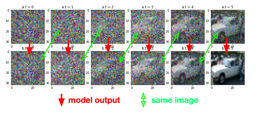
这就是扩散模型的工作原理:它就像基于一个完全嘈杂的图像,并逐渐提高图像质量,直到它变得清晰。
(如下图所示)
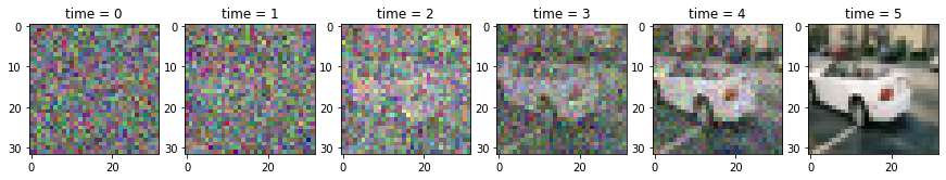
因此,我们可以创建一个深度学习模型,可以提高图像质量(从全噪声到清晰的图像),流程思想:
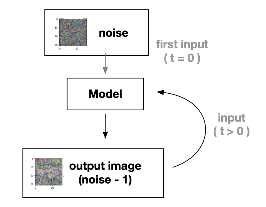
为了更清晰地了解,请查看此附加流程图。
如上图所示,该模型正在尝试生成噪声逐渐减少的图像。现在,我们只需要训练一个深度学习模型来学习如何减少噪音。
对于该任务,我们需要模型中的两个输入:
- 输入图像 — 需要处理噪声图像
- 时间戳 — 告诉模型什么是噪声状态,以便更容易学习
三、实现快速扩散模型
首先,让我们导入我们需要的内容:
import numpy as np

from tqdm.auto import trange, tqdm
import matplotlib.pyplot as plt

import tensorflow as tf
from tensorflow.keras import layers
并准备我们的数据集, 在本教程中,我们将使用大量汽车图像(CIFAR-10)作为示例,以使事情尽可能简单快捷。
(但是,如果您有足够的样本,则可以选择您喜欢的任何图像。
(X_train, y_train), (X_test, y_test) = tf.keras.datasets.cifar10.load_data()
X_train = X_train[y_train.squeeze() == 1]
X_train = (X_train / 127.5) - 1.0
接下来,让我们定义变量。
IMG_SIZE = 32     # input image size, CIFAR-10 is 32x32
BATCH_SIZE = 128  # for training batch size
timesteps = 16    # how many steps for a noisy image into clear
time_bar = 1 - np.linspace(0, 1.0, timesteps + 1) # linspace for timesteps
在这里,我们设置“时间步长”,这意味着我们的模型将学习通过训练过程生成从嘈杂(级别 0)到清晰(级别 16)的图像。
让我们看一张图片以获得更清晰的想法
plt.plot(time_bar, label='Noise')
plt.plot(1 - time_bar, label='Clarity')
plt.legend()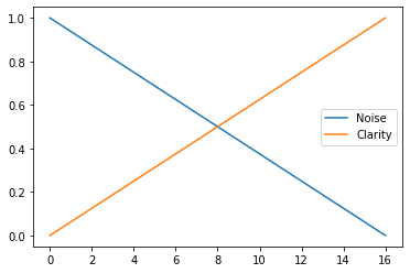
如您所见,从时间步长 0 到 16,噪音减少,清晰度逐渐提高。这就是我们希望我们的模型学习的内容。
并为预览数据准备一些功能
def cvtImg(img):
    img = img - img.min()
    img = (img / img.max())
    return img.astype(np.float32)

def show_examples(x):
    plt.figure(figsize=(10, 10))
    for i in range(25):
        plt.subplot(5, 5, i+1)
        img = cvtImg(x[i])
        plt.imshow(img)
        plt.axis('off')

show_examples(X_train)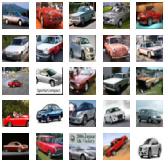
CIFAR-10 汽车
3.1 培训准备
在这里,我们需要准备训练图像的代码。
这个想法是从随机时间点获得两个图像(A和B),其中A是噪声图像,B是更清晰的图像。
我们的模型将学习根据该特定时间点将A转换为B(从嘈杂到更清晰)。
(再次作为此图)
因此,我们在这里forward_noise功能。
def forward_noise(x, t):
a = time_bar[t] # base on t
b = time_bar[t + 1] # image for t + 1
noise = np.random.normal(size=x.shape) # noise mask
a = a.reshape((-1, 1, 1, 1))
b = b.reshape((-1, 1, 1, 1))
img_a = x * (1 - a) + noise * a
img_b = x * (1 - b) + noise * b
return img_a, img_b
def generate_ts(num):
return np.random.randint(0, timesteps, size=num)
# t = np.full((25,), timesteps - 1) # if you want see clarity
# t = np.full((25,), 0) # if you want see noisy
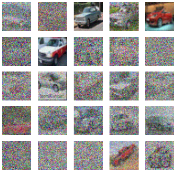
t = generate_ts(25) # random for training data
a, b = forward_noise(X_train[:25], t)
show_examples(a)如果你想了解它是如何工作的,我建议运行我注释掉的代码。( t = ... )
3.2 构建 CNN 块
我们将使用 U-Net 作为我们的模型,详细信息将在下面的代码中解释。
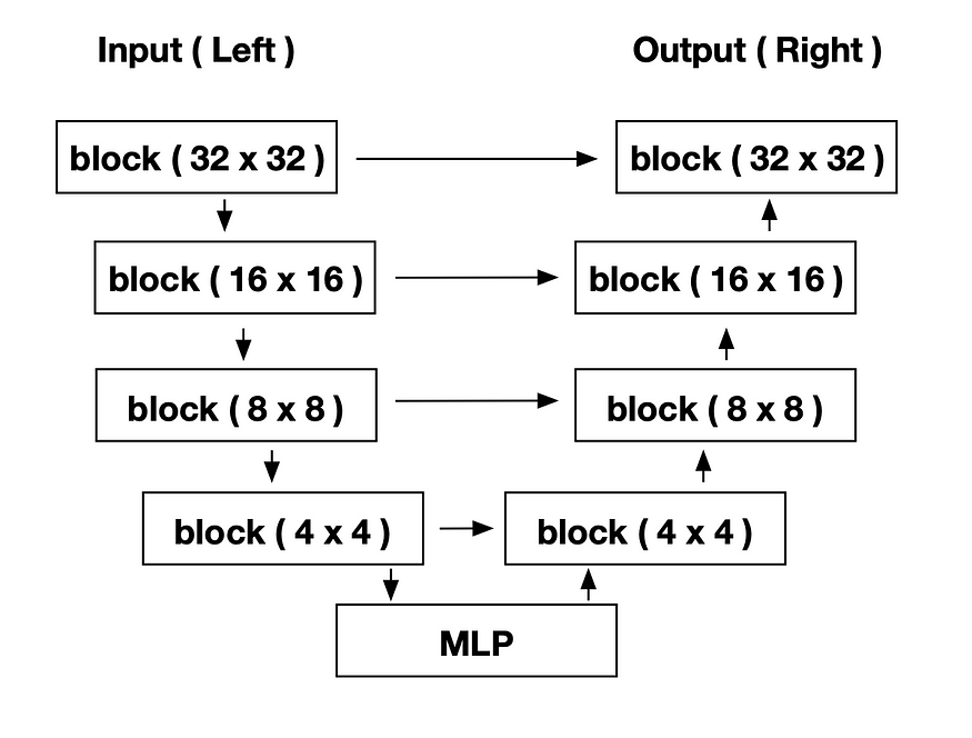
模型架构,详细内容会在后面的代码中讲解,在构建模型之前,我们需要先定义块。
这是 make 块的代码:
def block(x_img, x_ts):
x_parameter = layers.Conv2D(128, kernel_size=3, padding='same')(x_img)
x_parameter = layers.Activation('relu')(x_parameter)
time_parameter = layers.Dense(128)(x_ts)
time_parameter = layers.Activation('relu')(time_parameter)
time_parameter = layers.Reshape((1, 1, 128))(time_parameter)
x_parameter = x_parameter * time_parameter
# -----
x_out = layers.Conv2D(128, kernel_size=3, padding='same')(x_img)
x_out = x_out + x_parameter
x_out = layers.LayerNormalization()(x_out)
x_out = layers.Activation('relu')(x_out)
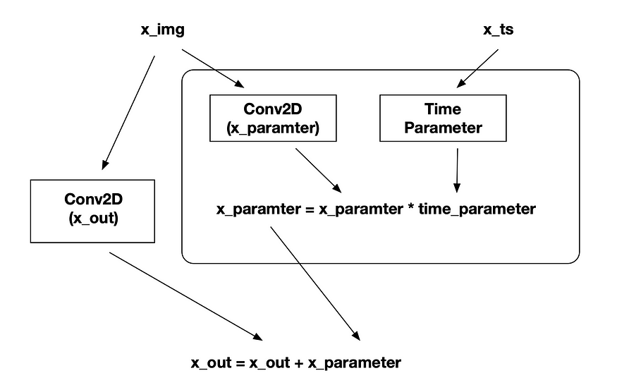
return x_out 每个块包含两个带有时间参数的卷积网络,允许网络确定其当前的时间步长并输出相应的信息。
您可以看到块流程图:
(x_img 是输入图像,是噪声图像,x_ts 是时间步长的输入)
搭建模型,现在我们可以构建我们的模型
def make_model():
    x = x_input = layers.Input(shape=(IMG_SIZE, IMG_SIZE, 3), name='x_input')

    x_ts = x_ts_input = layers.Input(shape=(1,), name='x_ts_input')
    x_ts = layers.Dense(192)(x_ts)
    x_ts = layers.LayerNormalization()(x_ts)
    x_ts = layers.Activation('relu')(x_ts)

    # ----- left ( down ) -----
    x = x32 = block(x, x_ts)
    x = layers.MaxPool2D(2)(x)

    x = x16 = block(x, x_ts)
    x = layers.MaxPool2D(2)(x)

    x = x8 = block(x, x_ts)
    x = layers.MaxPool2D(2)(x)

    x = x4 = block(x, x_ts)

    # ----- MLP -----
    x = layers.Flatten()(x)
    x = layers.Concatenate()([x, x_ts])
    x = layers.Dense(128)(x)
    x = layers.LayerNormalization()(x)
    x = layers.Activation('relu')(x)

    x = layers.Dense(4 * 4 * 32)(x)
    x = layers.LayerNormalization()(x)
    x = layers.Activation('relu')(x)
    x = layers.Reshape((4, 4, 32))(x)

    # ----- right ( up ) -----
    x = layers.Concatenate()([x, x4])
    x = block(x, x_ts)
    x = layers.UpSampling2D(2)(x)

    x = layers.Concatenate()([x, x8])
    x = block(x, x_ts)
    x = layers.UpSampling2D(2)(x)

    x = layers.Concatenate()([x, x16])
    x = block(x, x_ts)
    x = layers.UpSampling2D(2)(x)

    x = layers.Concatenate()([x, x32])
    x = block(x, x_ts)

    # ----- output -----
    x = layers.Conv2D(3, kernel_size=1, padding='same')(x)
    model = tf.keras.models.Model([x_input, x_ts_input], x)
    return model

model = make_model()
# model.summary()
这是一个U-Net,左、右、MLP部分可以参考上图(模型架构)。
不要忘记编译模型
optimizer = tf.keras.optimizers.Adam(learning_rate=0.0008)
loss_func = tf.keras.losses.MeanAbsoluteError()
model.compile(loss=loss_func, optimizer=optimizer)
我们使用 Adam 作为优化器,使用 MeanAbsoluteError (MAE) 作为损失函数。
预测结果:我们现在可以尝试我们的第一个预测。预测步骤如下:
- 创建嘈杂的图像
- 以时间步长输入到我们的模型中
- 继续这样做直到时间步结束
所以这是这个函数:
def predict(x_idx=None):
    x = np.random.normal(size=(32, IMG_SIZE, IMG_SIZE, 3))
    for i in trange(timesteps):
        t = i
        x = model.predict([x, np.full((32), t)], verbose=0)
    show_examples(x)

predict()
未经训练的模型输出图像 上面是我们的未经训练的模型输出,如您所见,它没有任何用处。 这个函数还可以帮助我们查看每个步骤:
def predict_step():
    xs = []
    x = np.random.normal(size=(8, IMG_SIZE, IMG_SIZE, 3))

    for i in trange(timesteps):
        t = i
        x = model.predict([x, np.full((8),  t)], verbose=0)
        if i % 2 == 0:
            xs.append(x[0])

    plt.figure(figsize=(20, 2))
    for i in range(len(xs)):
        plt.subplot(1, len(xs), i+1)
        plt.imshow(cvtImg(xs[i]))
        plt.title(f'{i}')
        plt.axis('off')

predict_step()
四、训练模型
这个训练功能很简单
def train_one(x_img):
    x_ts = generate_ts(len(x_img))
    x_a, x_b = forward_noise(x_img, x_ts)
    loss = model.train_on_batch([x_a, x_ts], x_b)
return loss我们只需要提供x_ts和x_img(x_a),使我们的模型能够学习如何生成x_b。
并使其成为纪元函数
def train(R=50):
    bar = trange(R)
    total = 100
    for i in bar:
        for j in range(total):
            x_img = X_train[np.random.randint(len(X_train), size=BATCH_SIZE)]
            loss = train_one(x_img)
            pg = (j / total) * 100
            if j % 5 == 0:
                bar.set_description(f'loss: {loss:.5f}, p: {pg:.2f}%')
最后,多次运行并逐渐降低学习率
for _ in range(10):
    train()
    # reduce learning rate for next training
    model.optimizer.learning_rate = max(0.000001, model.optimizer.learning_rate * 0.9)

    # show result
    predict()
    predict_step()
    plt.show()
你可以得到一些这样的输出图像

五、结论
本教程设计简单,允许您进行实验。您可以尝试自己的参数(如更改图像大小,CNN过滤器,时间步长或MLP等)和更多的时期训练以获得更好的结果。海沌