R手册(Visualise)--GGally(ggplot2 extensions)

- GGally

GGally

GGally通过添加几个函数来扩展ggplot2，以降低geom与转换数据组合的复杂性。其中一些功能包括配对图矩阵，散点图矩阵，平行坐标图，生存图，以及绘制网络的几个函数。

ggmatrix： ggplot2矩阵

用法

ggmatrix()

参数
plots：将要列入矩阵的图形列表
nrow, ncol：行数和列数
xAxisLabels, yAxisLabels：# x标签和y标签。设置NULL为不显示
title, xlab, ylab：标题，x标签和y标签。设置NULL为不显示
byrow：布尔值，用于确定图应该按行还是按列排序
showStrips：布尔值来确定是否应显示每个图块。NULL将仅默认为顶部和右侧地块。
showAxisPlotLabels, showXAxisPlotLabels, showYAxisPlotLabels：布尔值，用于确定绘图轴标签是否打印在绘图矩阵的X（底部）或Y（左侧）部分。

plotList <- list()
for (i in 1:6) {
  plotList[[i]] <- ggally_text(paste("Plot #", i, sep = ""))
}

pm <- ggmatrix(
  plotList,           #将要列入矩阵的图形列表
  nrow = 2, ncol = 3, # 行数和列数
  xAxisLabels = c("A", "B", "C"),  #x标题。设置NULL为不显示
  yAxisLabels = c("D", "E"),
  by
  title = "Matrix Title"
)
pm
pm <- pm + theme_bw()   #可以添加ggplot2主题
p2 <- pm[1,2]           #也可以提取子集使用
p3 <- pm[1,3]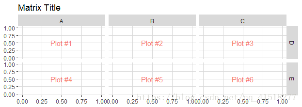

matrix

ggpairs：ggplot2广义配对图

选定列映射

data(tips, package = "reshape")
pm <- ggpairs(tips, mapping = aes(color = sex), 
  columns = c("total_bill", "time", "tip"),columnLabels = c("Total Bill", "Time of Day", "Tip"))
pm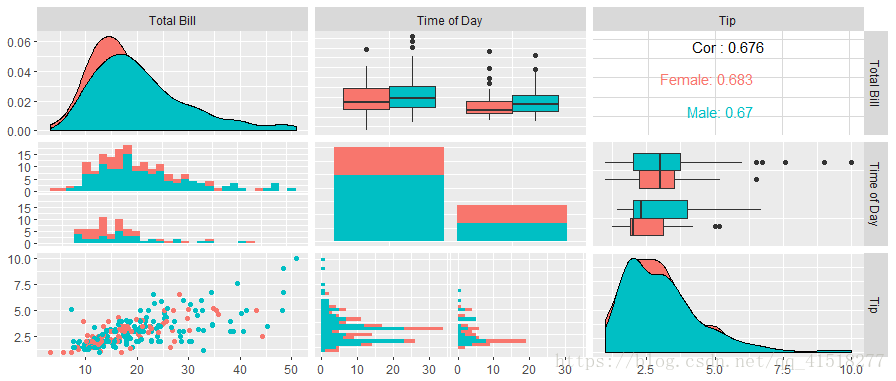

矩阵部分
成对矩阵有三个主要部分：lower，upper，和diag。lower和upper包含三个类型：continuous，combo，和discrete。diag只包含continuous或者discrete。

continuous：X和Y都是连续变量
combo：一个是离散的，而另一个是连续的
discrete：X和Y都是离散变量

要对每个部分进行调整，需要提供一个信息列表。该列表可以由以下元素组成：

continuous：
- 表示ggally_NAME函数尾部的字符串或自定义函数
- 当前有效的upper$continuous和lower$continuous字符串：’points’，’smooth’，’density’，’cor’，’blank’
- 当前有效的diag$continuous字符串：’densityDiag’，’barDiag’，’blankDiag’
combo：
表示ggally_NAME函数尾部的字符串或自定义函数。（不适用于diag列表）
当前有效的upper$combo和lower$combo字符串：’box’，’dot’，’facethist’，’facetdensity’，’denstrip’，’blank’
discrete：
- 表示ggally_NAME函数尾部的字符串或自定义函数
- 当前有效的upper$discrete和lower$discrete字符串：’ratio’，’facetbar’，’blank’
- 当前有效的diag$discrete字符串：’barDiag’，’blankDiag’
mapping：如果提供了映射，则只会覆盖该部分的映射

library(ggplot2)
pm <- ggpairs(
  tips, columns = c("total_bill", "time", "tip"),
  lower = list(
    continuous = "smooth",
    combo = "facetdensity",
    mapping = aes(color = time)
  )
)
pm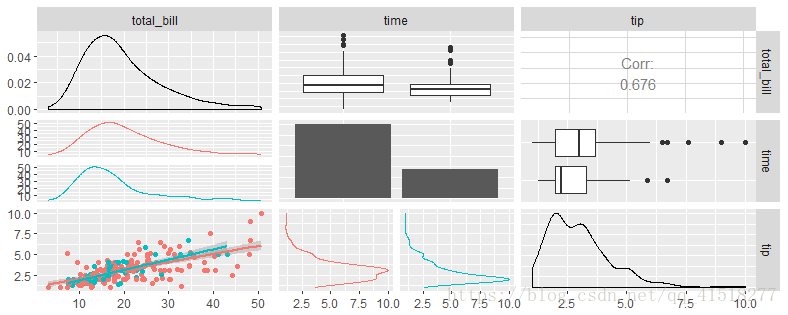

自定义函数
这些ggally_NAME函数不提供所有图形选项。一个自定义函数可以代替供给字符串到continuous，combo或discrete内的元件upper，lower或diag。

自定义函数应该遵循：只要返回一个ggplot2对象即可

custom_function <- function(data, mapping, ...){
  # produce ggplot2 object here
}

my_bin <- function(data, mapping, ..., low = "#132B43", high = "#56B1F7") {
  ggplot(data = data, mapping = mapping) +
    geom_bin2d(...) +
    scale_fill_gradient(low = low, high = high)
}
pm <- ggpairs(
  tips, columns = c("total_bill", "time", "tip"),
  lower = list(
    continuous = my_bin
  )
)
pm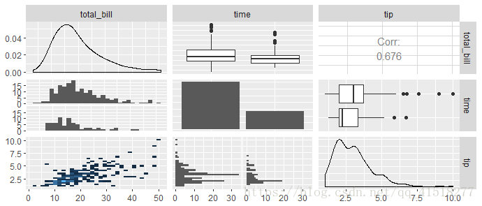

函数包装
上面的例子使用每个子图的默认参数。要更改默认的参数binwidth设置，我们将使用wrap函数。wrap第一个参数是一个字符串或一个自定义函数。提供给wrap的其余参数将在运行时提供给函数。

pm <- ggpairs(
  tips, columns = c("total_bill", "time", "tip"),
  lower = list(
    combo = wrap("facethist", binwidth = 1),
    continuous = wrap(my_bin, binwidth = c(5, 0.5), high = "red")
  )
)
pm

取矩阵子集和添加主题

p <- pm[3,1]  # 取子集
p <- p + aes(color = time)
p + theme_bw() #添加主题

ggscatmat：纯粹定量变量的传统散点图矩阵

ggscatmat(data, columns = 1:ncol(data), color = NULL, alpha = 1, corMethod = "pearson")

比ggpairs更快，因为需要做出更少的选择。它创建了一个矩阵，其中包含对角线下的散点图，对角线的密度图以及对角线上的相关系数。

data(flea)
ggscatmat(flea, columns = 2:4, color="species", alpha=0.8)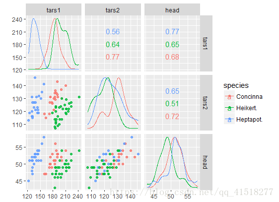

其余函数待更新