利用流型的优化方法（manifold optimization）

方法简要总结

什么是流型

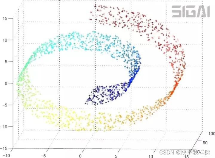
流形（manifold）是几何中的一个概念，它是高维空间中的几何结构，即空间中的点构成的集合。可以简单的将流形理解成二维空间的曲线，三维空间的曲面在更高维空间的推广。下图是三维空间中的一个流形，这是一个卷曲面：

针对RIS相位优化的子问题

介绍下面论文中的优化方法
https://ieeexplore.ieee.org/stamp/stamp.jsp?tp=&arnumber=9090356
Recall that ${\varphi }_m=e^{j{\theta }_m},\forall m$, and that $\mathbf{\varphi }={\left[{\varphi }_1,\cdots ,{\varphi }_M\right]}^{\mathrm{T}}$
$$\begin{array}{l}{\min }_{\mathbf{\varphi }}f(\mathbf{\varphi })\triangleq {\mathbf{\varphi }}^{\mathrm{H}}\mathbf{\Xi }\mathbf{\varphi }+2\mathrm{Re}\left\{{\mathbf{\varphi }}^{\mathrm{H}}{\mathbf{v}}^{\ast }\right\}\\ \text{ s.t. }\left|{\varphi }_m\right|=1,m=1,\cdots ,M.\end{array}\text{\hspace{1em}(35)}$$

MM方法

见我之前的博客记录方法

Complex Circle Manifold (CCM) Method

在本小节中，我们采用文[35]中提出的CCM方法直接求解问题（35）。 我们首先将问题（35）转化为下面的等价问题

$$\begin{array}{l}{\min }_{\varphi }\bar{f}(\varphi )\triangleq {\varphi }^{\mathrm{H}}\left(\mathbf{\Xi }+\alpha {\mathbf{I}}_M\right)\varphi +2\mathrm{Re}\left\{{\varphi }^{\mathrm{H}}{\mathbf{v}}^{\ast }\right\}\\ \text{ s.t. }\left|{\varphi }_m\right|=1,m=1,\cdots ,M\end{array}\text{\hspace{1em}(41)}$$
其中$\alpha >0$是一个正常数参数，其值将在定理1中给出。 问题（35）与问题（41）等价，因为我们有$\alpha {\varphi }^{\mathrm{H}}\mathbf{\varphi }=\alpha M$。 参数$\alpha$可以控制CCM方法的收敛性，这将在定理1中讨论。
问题（41）中的搜索空间可以看作the
product of $M$ complex circles(Each complex circle is given by S ≜ { x ∈ C : x ∗ x = Re ⁡ { x } 2 + Im ⁡ { x } 2 = 1 } \mathcal{S} \triangleq\left\{x \in \mathbb{C}: x^{*} x=\operatorname{Re}\{x\}^{2}+\right.\left.\operatorname{Im}\{x\}^{2}=1\right\} S≜{ x∈C:x∗x=Re{ x}2+Im{ x}2=1}
which is a sub-manifold of C [35])，它是${\mathbb{C}}^M$的子流形，由
$${\mathcal{S}}^M\triangleq \left\{\mathbf{x}\in {\mathbb{C}}^M:\left|x_l\right|=1,l=1,2,\cdots ,M\right\}\text{\hspace{1em}(42)}$$
where $x_l$ is the $l$th element of vector $\mathbf{x}$

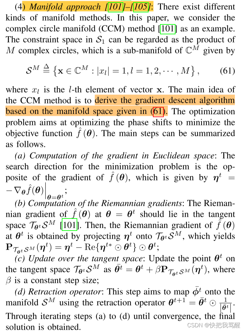
CCM算法的主要思想是基于（42）定义的流形空间推导出梯度下降算法，它类似于在欧几里得空间上为传统优化开发的梯度下降技术的概念。 CCM算法的主要步骤由每次迭代T中的四个主要步骤组成：

Step1 Gradient in Euclidean Space

我们首先要找到搜索方向，对于极小化问题，最常见的搜索方向是向与$\bar{f}\left({\varphi }^t\right)$梯度相反的方向移动，该方向由

$${\mathbf{\eta }}^t=-{\nabla }_{\mathbf{\varphi }}\bar{f}\left({\mathbf{\varphi }}^t\right)=-2\left(\mathbf{\Xi }+\alpha {\mathbf{I}}_M\right){\mathbf{\varphi }}^t-2{\mathbf{v}}^{\ast }\text{\hspace{1em}(43)}$$

Step2 Riemannian gradients:

黎曼梯度与欧几里得梯度是相对并列的概念：

由于我们在流形空间上进行优化，我们必须找到黎曼梯度[12]。$\bar{f}\left({\varphi }^t\right)$在当前点${\varphi }^t\in {\mathcal{S}}^M$处的黎曼梯度是在切空间${\mathcal{T}}_{{\varphi }^t}{\mathcal{S}}^M$中($\mathcal{S}$在点$z_m$处的切空间定义为 T z m S = { x ∈ C : Re ⁡ { x ∗ z m } = 0 } \mathcal{T}_{z_{m}} \mathcal{S}=\{x \in \mathbb{C}:\left.\operatorname{Re}\left\{x^{*} z_{m}\right\}=0\right\} Tzm​​S={ x∈C:Re{ x∗zm​}=0}。 则切空间${\mathcal{T}}_{\mathbf{z}}{\mathcal{S}}^M$是由${\mathcal{T}}_{\mathbf{z}}{\mathcal{S}}^M={\mathcal{T}}_{z_1}\mathcal{S}\times {\mathcal{T}}_{z_2}\mathcal{S}\cdots \times {\mathcal{T}}_{z_M}\mathcal{S}$给出的$M$个切空间${\mathcal{T}}_{z_m}\mathcal{S}$的乘积) 。具体地说，将欧氏空间中的搜索方向${\mathbf{\eta }}^t$用投影算子投影到${\mathcal{T}}_{{\varphi }^t}{\mathcal{S}}^M$上，就可以得到$\bar{f}\left({\varphi }^t\right)$在${\varphi }^t$处的黎曼梯度，其计算方法如下[12]:
$${\mathbf{P}}_{{\mathcal{T}}_{{\varphi }^t}{\mathcal{S}}^M}\left({\mathbf{\eta }}^t\right)={\mathbf{\eta }}^t-\mathrm{Re}\left\{{\mathbf{\eta }}^{t\ast }\odot {\mathbf{\varphi }}^t\right\}\odot {\mathbf{\varphi }}^t\text{\hspace{1em}(44)}$$

Step3 Update over the tangent space

在切空间( tangent space)上更新：在切空间${\mathcal{T}}_{{\varphi }^t}{\mathcal{S}}^M$上更新当前点${\mathbf{\varphi }}^t$:

$${\bar{\varphi }}^t={\varphi }^t+\beta {\mathbf{P}}_{{\mathcal{T}}_{{\varphi }^t}{\mathcal{S}}^M}\left({\mathbf{\eta }}^t\right)\text{\hspace{1em}(45)}$$

其中β是常数步长，将在定理1中讨论。

Step4 Retraction operator

一般情况下，得到的${\bar{\varphi }}^t$不在${\mathcal{S}}^M$中，即。 我们有${\bar{\varphi }}^t\notin {\mathcal{S}}^M$。 因此，必须通过如下使用缩回操作器(缩回运算符将${\bar{\varphi }}^t$的每个元素归一化为单位值。)将其映射到流形${\mathcal{S}}^M$中

$${\varphi }^{t+1}={\bar{\varphi }}^t\odot \frac{1}{\left|{\bar{\varphi }}^t\right|}\text{\hspace{1em}(46)}$$

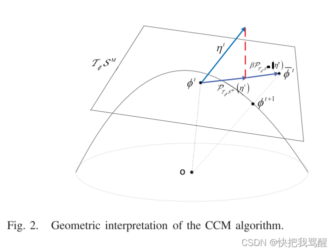
注意，${\bar{\varphi }}^{t+1}$和${\bar{\varphi }}^t$都属于满足单位常数模约束的${\mathcal{S}}^M$。 CCM算法的细节在算法3中给出。 CCM算法在Fig2中也得到了几何学的说明. 下面的定理为参数α和β的选择提供了指导，以保证CCM算法的收敛性。

Theorem 1 [35]: Let ${\lambda }_{\mathbf{\Xi }}$ and ${\lambda }_{\mathbf{\Xi }+\alpha \mathbf{I}}$
be the largest eigenvalue of matrices $\mathbf{\Xi }$ and $\mathbf{\Xi }+\alpha \mathbf{I}$, respectively. If α and β
are chosen to satisfy the following condition：

$$\alpha \ge \frac{M}{8}{\lambda }_{\mathbf{\Xi }}+\Vert \mathbf{v}{\Vert }_2,0<\beta <\frac{1}{{\lambda }_{\mathbf{\Xi }+\alpha \mathbf{I}}}\text{\hspace{1em}(47)}$$

then the CCM algorithm generates a non-increasing sequence
$\left\{\bar{f}\left({\varphi }^t\right),t=1,2,\cdots \right\}$, and finally converges to a finite
value.


some code

一些关于CCM优化 An-Overview-of-Signal-Processing-Techniques-for-RIS-IRS-aided-Wireless-Systems的作者放在GitHub的代码（不是我写的，仅供参考）：

function [e_opt,obj_e] = Generate_beamforming_e(N, M, K, G_tilde, z, W, e_ini, noise, power)

%%  Generate the parameters  %%%%%
A = zeros(size(G_tilde,2),size(G_tilde,2));
a = zeros(size(G_tilde,2),1);
for k = 1 : K
    A = A + abs( z(k) )^2 * G_tilde(:,:,k)' * W * W' * G_tilde(:,:,k);
    a = a + ( z(k) * W(:,k).' * conj( G_tilde(:,:,k) ) )';
end
e_tilde  = [e_ini;1];

% 黎曼梯度与欧几里得梯度
grad_euc = - ( A.' * e_tilde - a );
grad_Rie = grad_euc - real( conj( grad_euc ) .* e_tilde ) .* e_tilde;
beta = 100;
% tang域值，并归一化
e_tang   = e_tilde + beta * grad_Rie;
e_opt    = e_tang(1:M) ./ abs(e_tang(1:M));
ee    = [ e_opt; 1 ];
obj_e = ee' * A.' * ee - 2 * real( a' * ee ) + noise * z' * z + K;
end

close all;
clear all;clc;
warning('off');
rand('twister',mod(floor(now*8640000),2^31-1));

N          = 10;            % array number of BS
M_all      = 10:10:100;            % array number of IRS
K          = 4;            % number of users in each group

SNR        = 5;     % dBm
noise      = 1; % W
power      = 10^(SNR/10)*noise;


%% Simulation loop %%%%%%%%%%%%%%%%%%%%%%%%%%%%%%%%%%%%%%%%%%%%%%
num_loop = 1000; 
for loop = 1 : num_loop
    outerflag=1; 
    for m = 1 : length(M_all)
        t0 = cputime;
        M  = M_all(m);
        %%%%%  Generate channel  %%%%%
        H   = (1/sqrt(2)) * ( randn(N,M) + 1i*randn(N,M) );
        H   = H / norm( H, 'fro' ) * sqrt( N * M );
        h_r = (1/sqrt(2)) * ( randn(M,K) + 1i*randn(M,K) );
        h_r = h_r / norm( h_r, 'fro' ) * sqrt( K * M );
        h_d = (1/sqrt(2)) * ( randn(N,K) + 1i*randn(N,K) );
        h_d = h_d / norm( h_d, 'fro' ) * sqrt( K * M );
        G=[];  G_tilde=[];
        for k=1:K
            G(:,:,k,m,loop)       = H * diag(h_r(:,k));
            G_tilde(:,:,k,m,loop) = [G(:,:,k,m,loop) h_d(:,k)];
        end
    end
end
save('G','G');
save('G_tilde','G_tilde');

%By Zhou Gui
%From 2019-2-14 to 
close all;
clear all;clc;
warning('off');
rand('twister',mod(floor(now*8640000),2^31-1));
%% Parameters Initialization %%%%%%%%%%%%%%%%%%%%%%%%%%%%%%%%%%%%%
% '1' stands for source-relays; '2' stands for relays-destination
N          = 10;            % array number of BS
M_all      = 100:10:100;            % array number of IRS
K          = 4;            % number of users in each group

SNR        = 5;     % dBm
noise      = 1; % W
power      = 10^(SNR/10)*noise;


%% Simulation loop %%%%%%%%%%%%%%%%%%%%%%%%%%%%%%%%%%%%%%%%%%%%%%
num_loop = 100; 
for loop = 1 : num_loop
    outerflag=1; 
for m = 1 : length(M_all)
    t0 = cputime;
    M  = M_all(m);
    %%%%%  Generate channel  %%%%%
    H   = (1/sqrt(2)) * ( randn(N,M) + 1i*randn(N,M) );
    H   = H / norm( H, 'fro' ) * sqrt( N * M );
    h_r = (1/sqrt(2)) * ( randn(M,K) + 1i*randn(M,K) );
    h_r = h_r / norm( h_r, 'fro' ) * sqrt( K * M );
    h_d = (1/sqrt(2)) * ( randn(N,K) + 1i*randn(N,K) );
    h_d = h_d / norm( h_d, 'fro' ) * sqrt( K * M );
    G=[];  G_tilde=[];
    for k=1:K
        G(:,:,k)       = H * diag(h_r(:,k));
        G_tilde(:,:,k) = [G(:,:,k) h_d(:,k)];
    end

    %%%%%  Initialization  %%%%% 
    e_ini = [];  e_ini    = ones(M,1);
%     e_ini = [];  e_ini    = exp(1j*angle((1/sqrt(2)) * ( randn(M,1) + 1i*randn(M,1) )));
    W_ini = [];  W_ini    = ones(N,K)*sqrt(power/(N*K)); 
    W     = [];  W(:,:,1) = W_ini;
    e     = [];  e(:,1)   = e_ini;
    
    num_iterative = 10000;
    for n  = 1 : num_iterative
       %%%%%  Optimize a  %%%%%
       for k=1:K
           gk(:,k) = G_tilde(:,:,k)*[ conj(e(:,n)); 1];
           z(k,1)  = W(:,k,n)' * gk(:,k) / ( gk(:,k)'*W(:,:,n)*W(:,:,n)'*gk(:,k) + noise );
       end
       
       %%%%%  Optimize W  %%%%%
       P   = gk*diag(z');
       F_0 = inv(P*P')*P;
       if norm(F_0,'fro')^2 <= power
          F = F_0;
       else
          lambda_max = 20;
          lambda_min = 0;
          while   (lambda_max-lambda_min) > 10^(-5)
              lambda     = ( lambda_max + lambda_min ) / 2;
              F = inv(P*P' + lambda*eye(N))*P;
              if norm(F,'fro')^2 > power 
                 lambda_min = lambda;
              else if norm(F,'fro')^2 < power 
                      lambda_max = lambda;
                  end
              end
          end
       end
       W(:,:,n+1) = F;
       
       
       %%%%%  Optimize e  %%%%%
        [e_opt,obj] = Generate_beamforming_e(N, M, ...
                        K, G_tilde, z, W(:,:,n+1), e(:,n), noise, power);
        obj_e(n+1)=obj;
        e(:,n+1)=e_opt;
    
        %%%%%  stop criterion  %%%%%
        if abs(obj_e(n+1)-obj_e(n))<10^(-7)
            break;
        end
        x=[loop,m,n]
    end
 
    %%%%%  Generate rate  %%%%%
    F = W(:,:,n+1);
    e_tilde = [ e(:,n+1); 1 ];
    rate=0;
    for k=1:K
        temp = F(:,k)' * G_tilde(:,:,k) * conj( e_tilde );
        r(k) = e_tilde.' *G_tilde(:,:,k)' * F * F' * G_tilde(:,:,k) * conj( e_tilde ) + noise;
        r_g(k) = r(k) - temp' * temp;
        rate = rate + log2( 1 + temp'*temp / r_g(k) );
    end
    Rate(loop,m)=real(rate);

    t2=cputime;
    CPU_Time(loop,m)=t2-t0;
end
    save('Rate','Rate');
    save('CPU_Time','CPU_Time');
end
a=1;