前言
齿轮及齿轮箱作为机械设备常用的调节转速和传递转矩的旋转机械设备,不仅能够传递较大的功率和载荷,而且具有较好的可靠性。但是在高精度的切削加工中,当齿轮在变转速、变载荷等复杂工况下工作,极易受到损伤、产生磨损、断齿等情况,使得加工精度大打折扣。因此,齿轮的状态监测和故障诊断变得尤为重要。
一、什么是多尺度排列熵?
排列熵是由 BANDT C 等提出的一种衡量一维时间序列复杂度的平均熵参数,常用来提取机械故障的特征。但齿轮及齿轮箱运转过程中的故障特征信息分布在多尺度中,仅用单一尺度的排列熵进行分析,会遗漏其余尺度上的故障特征信息。排列熵( Permutation Entropy,PE) 是一种度量时间序列复杂度和检测动力学突变的平均熵函数,算法简单,计算速度快。信号中由故障引起的高频冲击成分越多,排列熵值就越大。因此很多论文中引入排列熵指标作为评价不同滤波器长度滤波效果好坏的标准。
针对排列熵的不足,COSTA M 等提出了多尺度排列熵的概念。多尺度排列熵是在排列熵的基础上将时间序列进行多尺度粗粒化,然后计算不同尺度下粗粒化序列的排列熵,具体计算过程如下:

二、实验平台照片
为了验证本文所提方法的有效性,在实验平台下( 图2) ,采集试验台减速箱齿轮不同状态下的实时振动信号。齿轮减速箱型号为 JZQ200,采样频率为 8 200 Hz。选择齿轮正常、不平衡、松动、错位、断齿、裂痕这 6 种不同状态的数据进行实验验证。 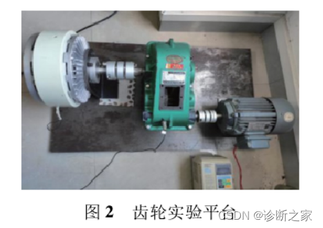
三、MATLAB代码
3.1 多尺度排列熵
function [pe hist] = pec(y,m,t)

%  Calculate the permutation entropy

%  Input:   y: time series;
%           m: order of permuation entropy
%           t: delay time of permuation entropy,

% Output:
%           pe:    permuation entropy
%           hist:  the histogram for the order distribution


ly = length(y);
permlist = perms(1:m);
c(1:length(permlist))=0;

 for j=1:ly-t*(m-1)
     [a,iv]=sort(y(j:t:j+t*(m-1)));
     for jj=1:length(permlist)
         if (abs(permlist(jj,:)-iv))==0
             c(jj) = c(jj) + 1 ;
         end
     end
 end

hist = c;

c=c(find(c~=0));
p = c/sum(c);
pe = -sum(p .* log(p));
function outdata = PE( indata, delay, order, windowSize )
% @brief PE efficiently [1] computes values of permutation entropy [2] in
% maximally overlapping sliding windows
%
% INPUT
%   - indata - considered time series
%   - delay - delay between points in ordinal patterns (delay = 1 means successive points)
%   - order - order of the ordinal patterns (order+1 - number of points in ordinal patterns)
%   - windowSize - size of sliding window
% OUTPUT
%   - outdata - values of normalised permutation entropy as defined in [2]
%
% REFERENCES
% [1] Unakafova, V.A., Keller, K., 2013. Efficiently measuring complexity
% on the basis of real-world data. Entropy, 15(10), 4392-4415.
% [2] Bandt C., Pompe B., 2002. Permutation entropy: a natural complexity
% measure for time series. Physical review letters, APS
%
% @author Valentina Unakafova
% @date 10.11.2017
% @email UnakafovaValentina(at)gmail.com

 load( ['table' num2str( order ) '.mat'] ); % the precomputed table
 patternsTable = eval( ['table' num2str( order )] );
 nPoints    = numel( indata );              % length of the time series
 opOrder1   = order + 1;
 orderDelay = order*delay;
 nPatterns  = factorial( opOrder1 );   % amount of ordinal patterns
 patternsDistribution = zeros( 1, nPatterns ); % distribution of ordinal patterns
 outdata = zeros( 1, nPoints );        % values of permutation entropy
 inversionNumbers = zeros( 1, order ); % inversion numbers of ordinal pattern (i1,i2,...,id)
 prevOP = zeros( 1, delay );           % previous ordinal patterns for 1:opDelay
 ordinalPatternsInWindow = zeros( 1, windowSize ); % ordinal patterns in the window
 ancNum = nPatterns./factorial( 2:opOrder1 );  % ancillary numbers
 peTable( 1:windowSize ) = -( 1:windowSize ).*log( 1:windowSize  ); % table of precomputed values
 peTable( 2:windowSize ) = ( peTable( 2:windowSize ) - peTable( 1:windowSize - 1 ) )./windowSize;
 for iTau = 1:delay
     cnt = iTau;
     inversionNumbers( 1 ) = ( indata( orderDelay + iTau - delay ) >= indata( orderDelay + iTau ) );
     for j = 2:order
         inversionNumbers( j ) = sum( indata( ( order - j )*delay + iTau ) >= ...
           indata( ( opOrder1 - j )*delay + iTau:delay:orderDelay + iTau ) );
     end
     ordinalPatternsInWindow( cnt ) = sum( inversionNumbers.*ancNum ); % first ordinal patterns
     patternsDistribution( ordinalPatternsInWindow( cnt )+ 1 ) = ...
       patternsDistribution( ordinalPatternsInWindow( cnt ) + 1 ) + 1;
     for j = orderDelay + delay + iTau:delay:windowSize + orderDelay   % loop for the first window
         cnt = cnt + delay;
         posL = 1; % the position of the next point
         for i = j - orderDelay:delay:j - delay
             if( indata( i ) >= indata( j ) )
                 posL = posL + 1;
             end
         end
         ordinalPatternsInWindow( cnt ) = ...
           patternsTable( ordinalPatternsInWindow( cnt - delay )*opOrder1 + posL );
         patternsDistribution( ordinalPatternsInWindow( cnt ) + 1 ) = ...
           patternsDistribution( ordinalPatternsInWindow( cnt ) + 1 ) + 1;
     end
     prevOP( iTau ) = ordinalPatternsInWindow( cnt );
 end
 ordDistNorm = patternsDistribution/windowSize;
 tempSum = 0;
 for iPattern = 1:nPatterns
   if ( ordDistNorm( iPattern ) ~= 0 )
     tempSum = tempSum - ordDistNorm( iPattern )*log( ordDistNorm( iPattern ) );
   end
 end
 outdata( windowSize + delay*order ) = tempSum;

 iTau = mod( windowSize, delay ) + 1;   % current shift 1:delay
 patternPosition = 1;                   % position of the current pattern in the window
 for t = windowSize + delay*order + 1:nPoints % loop over all points
     posL = 1;                          % the position of the next point
     for j = t-orderDelay:delay:t-delay
         if( indata( j ) >= indata( t ) )
             posL = posL + 1;
         end
     end
     nNew = patternsTable( prevOP( iTau )*opOrder1 + posL ); % incoming ordinal pattern
     nOut = ordinalPatternsInWindow( patternPosition );      % outcoming ordinal pattern
     prevOP( iTau ) = nNew;
     ordinalPatternsInWindow( patternPosition ) = nNew;
     nNew = nNew + 1;
     nOut = nOut + 1;
     if ( nNew ~= nOut ) % update the distribution of ordinal patterns
         patternsDistribution( nNew ) = patternsDistribution( nNew ) + 1; % incoming ordinal pattern
         patternsDistribution( nOut ) = patternsDistribution( nOut ) - 1; % outcoming ordinal pattern
         outdata( t ) = outdata( t - 1 ) + ( peTable( patternsDistribution( nNew ) ) - ...
                                        peTable( patternsDistribution( nOut ) + 1  ) );
     else
         outdata( t ) = outdata( t - 1 );
     end
     iTau = iTau + 1;
     patternPosition = patternPosition + 1;
     if ( iTau > delay )
       iTau = 1;
     end
     if ( patternPosition > windowSize )
       patternPosition = 1;
     end
 end
 outdata = outdata( windowSize + delay*order:end )/log( factorial( order + 1 ) );
3.2 排列熵
%% 主函数调用模糊熵函数求时间序列的模糊熵值
clc;clear;
close all;
tic;
% 产生仿真信号
fs=100;   %数据采样率Hz
t=1:1/fs:4096*1/fs; %对数据进行采样
n = length(t);  %数据的采样数?
f1 =0.25; %信号的频率

f2=0.005;
x=2*sin(2*pi*f1*t+cos(2*pi*f2*t)); %产?原始信号
nt=0.2*randn(1,n); %?斯?噪声?成
y=x+nt; %含噪信号
% EEMD分解
Nstd=0.2;
NE=20;
X=eemd(y,Nstd,NE,100); % EEMD分解函数在本?的资源?可供下载
%%
% 相空间重构:eDim为嵌?维数
% 当X具有多列和多?时,每列将被视为独?的时间序列,该算法对X的每?列假设相同的嵌?维度和时间延迟,并以标量返回ESTDIM和ESTLAG。
[~,~,eDim] = phaseSpaceReconstruction(X');
% 求时间序列X的模糊熵,模糊熵的输?时间序列为?向量
X=X'; % 将信号y的各个分量转置
[m,n]=size(X);
r0=0.15; % r为相似容限度
Out_FuzEn=zeros(1,m);
for i=1:m
r=r0*std(X(i,:));
FuzEn(i) = FuzzyEntropy(X(i,:),eDim,r,2,1);
end
toc;
%% 模糊熵函数
function FuzEn = FuzzyEntropy(data,dim,r,n,tau)
%
% This function calculates fuzzy entropy (FuzEn) of a univariate signal data
%
% Inputs:
%
% data: univariate signal - a vector of size 1 x N (the number of sample points)
% dim: embedding dimension
% r: threshold (it is usually equal to 0.15 of the standard deviation of a signal - because we normalize signals to have a standard deviation of 1, here, r is usually equal to 0.15)
% n: fuzzy power (it is usually equal to 2)
% tau: time lag (it is usually equal to 1)
% 模糊熵算法的提出者:Chen Weiting,Wang Zhizhong,XieHongbo,et al. Characterization of surfaceEMG signal based on fuzzy entropy. IEEE Transactions on Neural Systems and Rehabilitation Engineering. 2007,15(2):266-272.
%
if nargin == 4, tau = 1; end
if nargin == 3, n = 2; tau=1; end
if tau > 1, data = downsample(data, tau); end
N = length(data);
result = zeros(1,2);
for m = dim:dim+1
count = zeros(N-m+1,1);
dataMat = zeros(N-m+1,m);
% 设置数据矩阵,构造成m维的?量
for i = 1:N-m+1
dataMat(i,:) = data(1,i:i+m-1);
end
% 利?距离计算相似模式数
for j = 1:N-m+1
% 计算切?雪夫距离,不包括?匹配情况
dataMat=dataMat-mean(dataMat,2);
tempmat=repmat(dataMat(j,:),N-m+1,1);
dist = max(abs(dataMat - tempmat),[],2);
D=exp(-(dist.^n)/r);
count(j) = (sum(D)-1)/(N-m);
end
result(m-dim+1) = sum(count)/(N-m+1);
end

% 计算得到的模糊熵值
FuzEn = log(result(1)/result(2));
end

%%
function [modos its]=eemd(x,Nstd,NR,MaxIter)
%--------------------------------------------------------------------------
%WARNING: this code needs to include in the same
%directoy the file emd.m developed by Rilling and Flandrin.
%This file is available at %http://perso.ens-lyon.fr/patrick.flandrin/emd.html
%We use the default stopping criterion.
%We use the last modification: 3.2007
% -------------------------------------------------------------------------
%  OUTPUT
%   modos: contain the obtained modes in a matrix with the rows being the modes
%   its: contain the iterations needed for each mode for each realization
%
%  INPUT
%  x: signal to decompose
%  Nstd: noise standard deviation
%  NR: number of realizations
%  MaxIter: maximum number of sifting iterations allowed.
% -------------------------------------------------------------------------
%   Syntax
%
%   modos=eemd(x,Nstd,NR,MaxIter)
%  [modos its]=eemd(x,Nstd,NR,MaxIter)
% -------------------------------------------------------------------------
%  NOTE:   if Nstd=0 and NR=1, the EMD decomposition is obtained.
% -------------------------------------------------------------------------
% EEMD was introduced in
% Wu Z. and Huang N.
% "Ensemble Empirical Mode Decomposition: A noise-assisted data analysis method".
% Advances in Adaptive Data Analysis. vol 1. pp 1-41, 2009.
%--------------------------------------------------------------------------
% The present EEMD implementation was used in
% M.E.TORRES, M.A. COLOMINAS, G. SCHLOTTHAUER, P. FLANDRIN,
%  "A complete Ensemble Empirical Mode decomposition with adaptive noise,"
%  IEEE Int. Conf. on Acoust., Speech and Signal Proc. ICASSP-11, pp. 4144-4147, Prague (CZ)
%
% in order to compare the performance of the new method CEEMDAN with the performance of the EEMD.
%
% -------------------------------------------------------------------------
% Date: June 06,2011
% Authors:  Torres ME, Colominas MA, Schlotthauer G, Flandrin P.
% For problems with the code, please contact the authors:
% To:  macolominas(AT)bioingenieria.edu.ar
% CC:  metorres(AT)santafe-conicet.gov.ar
% -------------------------------------------------------------------------
%  This version was run on Matlab 7.10.0 (R2010a)
%--------------------------------------------------------------------------

desvio_estandar=std(x);
x=x/desvio_estandar;
xconruido=x+Nstd*randn(size(x));
[modos, o, it]=emd(xconruido,'MAXITERATIONS',MaxIter);
modos=modos/NR;
iter=it;
if NR>=2
    for i=2:NR
        xconruido=x+Nstd*randn(size(x));
        [temp, ort, it]=emd(xconruido,'MAXITERATIONS',MaxIter);
        temp=temp/NR;
        lit=length(it);
        [p liter]=size(iter);
        if lit<liter
            it=[it zeros(1,liter-lit)];
        end;
        if liter<lit
            iter=[iter zeros(p,lit-liter)];
        end;

        iter=[iter;it];

        [filas columnas]=size(temp);
        [alto ancho]=size(modos);
        diferencia=alto-filas;
        if filas>alto
            modos=[modos; zeros(abs(diferencia),ancho)];
        end;
        if alto>filas
            temp=[temp;zeros(abs(diferencia),ancho)];
        end;

        modos=modos+temp;
    end;
end;
its=iter;
modos=modos*desvio_estandar;
end
参考文献
[1]韩雪飞, 施展, 华云松. 基于参数优化MOMEDA与CEEMDAN的滚动轴承微弱故障特征提取研究[J]. 机械强度.