动动发财的小手,点个赞吧!
针对任何领域微调预训练 NLP 模型的分步指南
简介
在当今世界,预训练 NLP 模型的可用性极大地简化了使用深度学习技术对文本数据的解释。然而,虽然这些模型在一般任务中表现出色,但它们往往缺乏对特定领域的适应性。本综合指南[1]旨在引导您完成微调预训练 NLP 模型的过程,以提高特定领域的性能。
动机
尽管 BERT 和通用句子编码器 (USE) 等预训练 NLP 模型可以有效捕获语言的复杂性,但由于训练数据集的范围不同,它们在特定领域应用中的性能可能会受到限制。当分析特定领域内的关系时,这种限制变得明显。
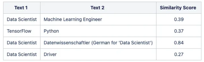
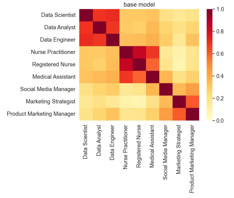
例如,在处理就业数据时,我们希望模型能够识别“数据科学家”和“机器学习工程师”角色之间的更接近,或者“Python”和“TensorFlow”之间更强的关联。不幸的是,通用模型常常忽略这些微妙的关系。
下表展示了从基本多语言 USE 模型获得的相似性的差异:
为了解决这个问题,我们可以使用高质量的、特定领域的数据集来微调预训练的模型。这一适应过程显着增强了模型的性能和精度,充分释放了 NLP 模型的潜力。
❝在处理大型预训练 NLP 模型时,建议首先部署基本模型,并仅在其性能无法满足当前特定问题时才考虑进行微调。
❞
本教程重点介绍使用易于访问的开源数据微调通用句子编码器 (USE) 模型。
可以通过监督学习和强化学习等各种策略来微调 ML 模型。在本教程中,我们将专注于一次(几次)学习方法与用于微调过程的暹罗架构相结合。
理论框架
可以通过监督学习和强化学习等各种策略来微调 ML 模型。在本教程中,我们将专注于一次(几次)学习方法与用于微调过程的暹罗架构相结合。
方法
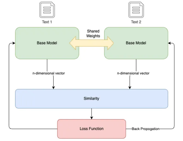
在本教程中,我们使用暹罗神经网络,它是一种特定类型的人工神经网络。该网络利用共享权重,同时处理两个不同的输入向量来计算可比较的输出向量。受一次性学习的启发,这种方法已被证明在捕获语义相似性方面特别有效,尽管它可能需要更长的训练时间并且缺乏概率输出。
连体神经网络创建了一个“嵌入空间”,其中相关概念紧密定位,使模型能够更好地辨别语义关系。
-
双分支和共享权重:该架构由两个相同的分支组成,每个分支都包含一个具有共享权重的嵌入层。这些双分支同时处理两个输入,无论是相似的还是不相似的。 -
相似性和转换:使用预先训练的 NLP 模型将输入转换为向量嵌入。然后该架构计算向量之间的相似度。相似度得分(范围在 -1 到 1 之间)量化两个向量之间的角距离,作为它们语义相似度的度量。 -
对比损失和学习:模型的学习以“对比损失”为指导,即预期输出(训练数据的相似度得分)与计算出的相似度之间的差异。这种损失指导模型权重的调整,以最大限度地减少损失并提高学习嵌入的质量。
数据概览
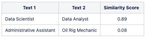
为了使用此方法对预训练的 NLP 模型进行微调,训练数据应由文本字符串对组成,并附有它们之间的相似度分数。
训练数据遵循如下所示的格式:
在本教程中,我们使用源自 ESCO 分类数据集的数据集,该数据集已转换为基于不同数据元素之间的关系生成相似性分数。
❝准备训练数据是微调过程中的关键步骤。假设您有权访问所需的数据以及将其转换为指定格式的方法。由于本文的重点是演示微调过程,因此我们将省略如何使用 ESCO 数据集生成数据的详细信息。
ESCO 数据集可供开发人员自由使用,作为各种应用程序的基础,这些应用程序提供自动完成、建议系统、职位搜索算法和职位匹配算法等服务。本教程中使用的数据集已被转换并作为示例提供,允许不受限制地用于任何目的。
❞
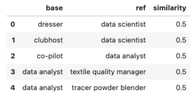
让我们首先检查训练数据:
import pandas as pd

# Read the CSV file into a pandas DataFrame
data = pd.read_csv("./data/training_data.csv")

# Print head
data.head()
起点:基线模型
首先,我们建立多语言通用句子编码器作为我们的基线模型。在进行微调过程之前,必须设置此基线。
在本教程中,我们将使用 STS 基准和相似性可视化示例作为指标来评估通过微调过程实现的更改和改进。
❝STS 基准数据集由英语句子对组成,每个句子对都与相似度得分相关联。在模型训练过程中,我们评估模型在此基准集上的性能。每次训练运行的持久分数是数据集中预测相似性分数和实际相似性分数之间的皮尔逊相关性。
这些分数确保当模型根据我们特定于上下文的训练数据进行微调时,它保持一定程度的通用性。
❞
# Loads the Universal Sentence Encoder Multilingual module from TensorFlow Hub.
base_model_url = "https://tfhub.dev/google/universal-sentence-encoder-multilingual/3"
base_model = tf.keras.Sequential([
    hub.KerasLayer(base_model_url,
                   input_shape=[],
                   dtype=tf.string,
                   trainable=False)
])

# Defines a list of test sentences. These sentences represent various job titles.
test_text = ['Data Scientist', 'Data Analyst', 'Data Engineer',
             'Nurse Practitioner', 'Registered Nurse', 'Medical Assistant',
             'Social Media Manager', 'Marketing Strategist', 'Product Marketing Manager']

# Creates embeddings for the sentences in the test_text list.
# The np.array() function is used to convert the result into a numpy array.
# The .tolist() function is used to convert the numpy array into a list, which might be easier to work with.
vectors = np.array(base_model.predict(test_text)).tolist()

# Calls the plot_similarity function to create a similarity plot.
plot_similarity(test_text, vectors, 90, "base model")

# Computes STS benchmark score for the base model
pearsonr = sts_benchmark(base_model)
print("STS Benachmark: " + str(pearsonr))
微调模型
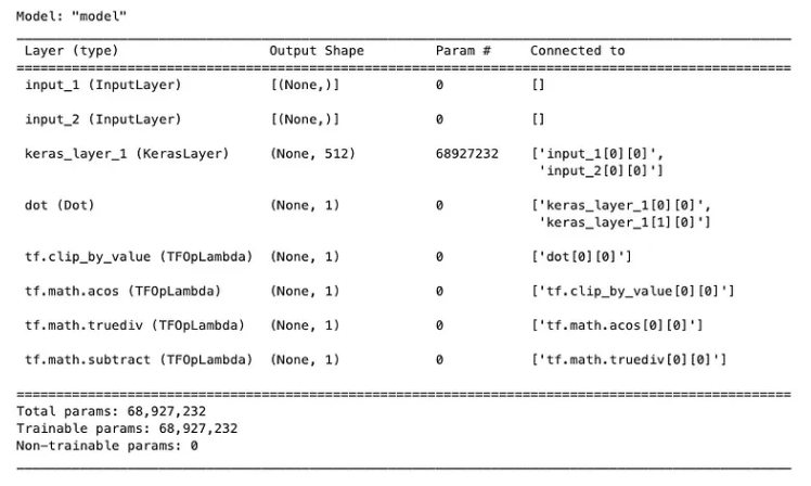
下一步涉及使用基线模型构建暹罗模型架构,并使用我们的特定领域数据对其进行微调。
# Load the pre-trained word embedding model
embedding_layer = hub.load(base_model_url)

# Create a Keras layer from the loaded embedding model
shared_embedding_layer = hub.KerasLayer(embedding_layer, trainable=True)

# Define the inputs to the model
left_input = keras.Input(shape=(), dtype=tf.string)
right_input = keras.Input(shape=(), dtype=tf.string)

# Pass the inputs through the shared embedding layer
embedding_left_output = shared_embedding_layer(left_input)
embedding_right_output = shared_embedding_layer(right_input)

# Compute the cosine similarity between the embedding vectors
cosine_similarity = tf.keras.layers.Dot(axes=-1, normalize=True)(
    [embedding_left_output, embedding_right_output]
)

# Convert the cosine similarity to angular distance
pi = tf.constant(math.pi, dtype=tf.float32)
clip_cosine_similarities = tf.clip_by_value(
    cosine_similarity, -0.99999, 0.99999
)
acos_distance = 1.0 - (tf.acos(clip_cosine_similarities) / pi)

# Package the model
encoder = tf.keras.Model([left_input, right_input], acos_distance)

# Compile the model
encoder.compile(
    optimizer=tf.keras.optimizers.Adam(
        learning_rate=0.00001,
        beta_1=0.9,
        beta_2=0.9999,
        epsilon=0.0000001,
        amsgrad=False,
        clipnorm=1.0,
        name="Adam",
    ),
    loss=tf.keras.losses.MeanSquaredError(
        reduction=keras.losses.Reduction.AUTO, name="mean_squared_error"
    ),
    metrics=[
        tf.keras.metrics.MeanAbsoluteError(),
        tf.keras.metrics.MeanAbsolutePercentageError(),
    ],
)

# Print the model summary
encoder.summary()
-
Fit model
# Define early stopping callback
early_stop = keras.callbacks.EarlyStopping(
    monitor="loss", patience=3, min_delta=0.001
)

# Define TensorBoard callback
logdir = os.path.join(".", "logs/fit/" + datetime.now().strftime("%Y%m%d-%H%M%S"))
tensorboard_callback = keras.callbacks.TensorBoard(log_dir=logdir)

# Model Input
left_inputs, right_inputs, similarity = process_model_input(data)

# Train the encoder model
history = encoder.fit(
    [left_inputs, right_inputs],
    similarity,
    batch_size=8,
    epochs=20,
    validation_split=0.2,
    callbacks=[early_stop, tensorboard_callback],
)

# Define model input
inputs = keras.Input(shape=[], dtype=tf.string)

# Pass the input through the embedding layer
embedding = hub.KerasLayer(embedding_layer)(inputs)

# Create the tuned model
tuned_model = keras.Model(inputs=inputs, outputs=embedding)
评估结果
现在我们有了微调后的模型,让我们重新评估它并将结果与基本模型的结果进行比较。
# Creates embeddings for the sentences in the test_text list.
# The np.array() function is used to convert the result into a numpy array.
# The .tolist() function is used to convert the numpy array into a list, which might be easier to work with.
vectors = np.array(tuned_model.predict(test_text)).tolist()

# Calls the plot_similarity function to create a similarity plot.
plot_similarity(test_text, vectors, 90, "tuned model")

# Computes STS benchmark score for the tuned model
pearsonr = sts_benchmark(tuned_model)
print("STS Benachmark: " + str(pearsonr))
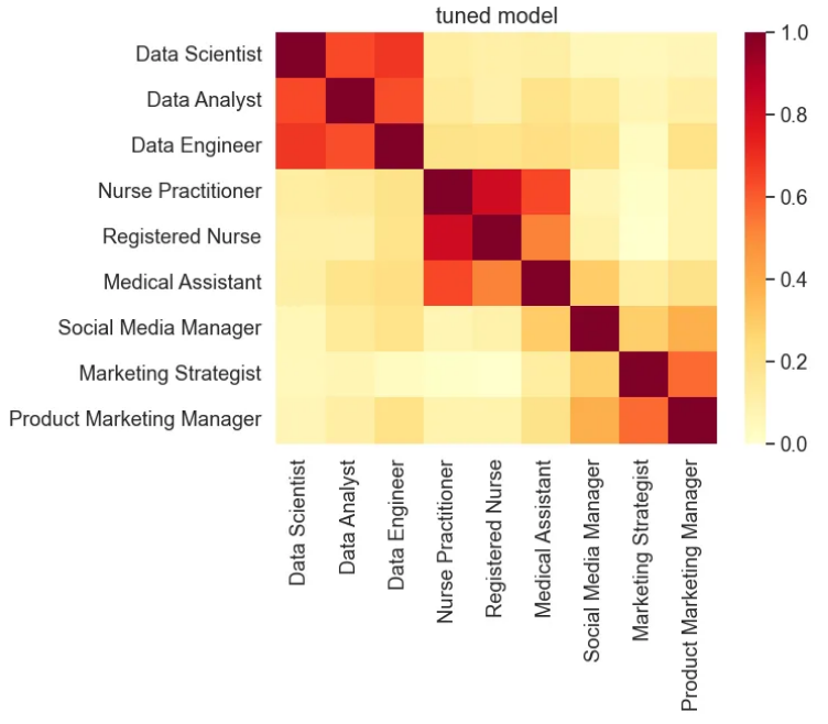
基于在相对较小的数据集上对模型进行微调,STS 基准分数与基线模型的分数相当,表明调整后的模型仍然具有普适性。然而,相似性可视化显示相似标题之间的相似性得分增强,而不同标题的相似性得分降低。
总结
微调预训练的 NLP 模型以进行领域适应是一种强大的技术,可以提高其在特定上下文中的性能和精度。通过利用高质量的、特定领域的数据集和暹罗神经网络,我们可以增强模型捕获语义相似性的能力。
本教程以通用句子编码器 (USE) 模型为例,提供了微调过程的分步指南。我们探索了理论框架、数据准备、基线模型评估和实际微调过程。结果证明了微调在增强域内相似性得分方面的有效性。
通过遵循此方法并将其适应您的特定领域,您可以释放预训练 NLP 模型的全部潜力,并在自然语言处理任务中取得更好的结果
Reference
Source: https://towardsdatascience.com/domain-adaption-fine-tune-pre-trained-nlp-models-a06659ca6668
本文由 mdnice 多平台发布