Datawhale202211—李宏毅《机器学习》(深度学习方向)
回归基本介绍+代码演示
文章目录
前言
随着人工智能的不断发展,机器学习这门技术也越来越重要,很多人都开启了学习机器学习,本系列文章就介绍了李宏毅老师《机器学习》基础内容。本文主要介绍回归相关的内容。
一、回归基本介绍
回归的定义
Regression 就是找到一个函数 functionfunction ,通过输入特征 x,输出一个数值 Scalar。
应用举例
- 股市预测(Stock market forecast)
输入:过去10年股票的变动、新闻咨询、公司并购咨询等
输出:预测股市明天的平均值- 自动驾驶(Self-driving Car)
输入:无人车上的各个sensor的数据,例如路况、测出的车距等
输出:方向盘的角度- 商品推荐(Recommendation)
输入:商品A的特性,商品B的特性
输出:购买商品B的可能性- Pokemon精灵攻击力预测(Combat Power of a pokemon):
输入:进化前的CP值、物种(Bulbasaur)、血量(HP)、重量(Weight)、
高度(Height)
输出:进化后的CP值
模型步骤
step1:模型假设-线性模型
- 首先,假设自变量和因变量之间的关系是线性的, 即可以表示为中元素的加权和,这里通常允许包含观测值的一些噪声;
- 其次,我们假设任何噪声都比较正常,如噪声遵循正态分布。
step2:模型评估-损失函数
损失函数(loss function)能够量化目标的实际值与预测值之间的差距。 通常我们会选择非负数作为损失,且数值越小表示损失越小,完美预测时的损失为0。
step3:最佳模型-梯度下降
通过不断地在损失函数递减的方向上更新参数来降低误差。梯度下降最简单的用法是计算损失函数(数据集中所有样本的损失均值) 关于模型参数的导数(在这里也可以称为梯度)。
模型优化
- 2个input的四个线性模型是合并到一个线性模型
- 更多参数,更多input
- 加入正则化
二、代码演示
import numpy as np
import matplotlib.pyplot as plt
from pylab import mpl # A tool used to draw 2D or 3D

# matplotlib没有中文字体,动态解决
plt.rcParams['font.sans-serif'] = ['Simhei']  # 显示中文
mpl.rcParams['axes.unicode_minus'] = False  # 解决保存图像是负号'-'显示为方块的问题
x_data = [338., 333., 328., 207., 226., 25., 179., 60., 208., 606.]
y_data = [640., 633., 619., 393., 428., 27., 193., 66., 226., 1591.]
x_d = np.asarray(x_data)
y_d = np.asarray(y_data)
# 区别array和asarray
- 相同点:array和asarray都能将结构数据转换成ndarray数组。
- 区别点:
(1)当他们的参数是列表型数据(list)时,二者没有区别;
(2)当他们的参数是数组类型(array)时,np.array()会返回参数数组的一个副本(copy,两者值一样但指向不同的内存),np.asarray()会返回参数数组的一个视图(两者指向同一块内存).- 优缺点:
(1)np.array()的副本会新开辟一块内存,对于大数组来说,会存在大量的复制操作,速度更慢且不节约内存;
(2)np.asarray()的视图相当于新增加了一个指向当前内存的引用,不存在复制操作,速度更快且节约内存。但是注意通过其中的一个引用修改数据,其他引用的数据也会跟着变,因为他们指向同一块内存区域。
x = np.arange(-200, -100, 1)
y = np.arange(-5, 5, 0.1)
Z = np.zeros((len(x), len(y)))
X, Y = np.meshgrid(x, y)
#print(X)
#print(Y)
解释一下meshgrid()
该函数返回一个坐标矩阵,首先该形式是矩阵,内容是坐标,用以描述一个网格。
- 给出一个坐标系的横纵坐标
- 横纵坐标形成一个网格
- 统计每个网格点的坐标,先横后竖,即可得到一个坐标矩阵
该示例描述如下:
X={[0,1,2],[0,1,2]}
Y={[1,1,1],[0,0,0]}
![X={[0,1,2],[0,1,2]} Y={[1,1,1],[0,0,0]](https://img-blog.csdnimg.cn/c77a6e3559d6404883e943d80eb3d457.png)
# loss
for i in range(len(x)):
    for j in range(len(y)):
        b = x[i]
        w = y[j]
        Z[j][i] = 0  # meshgrid吐出结果:y为行,x为列
        for n in range(len(x_data)):
            Z[j][i] += (y_data[n] - b - w * x_data[n]) ** 2
        Z[j][i] /= len(x_data)
# linear regression
#b = -120
#w = -4
b=-2
w=0.01
lr = 0.000005
iteration = 1400000

b_history = [b]
w_history = [w]
loss_history = []
import time
start = time.time()
for i in range(iteration):
    m = float(len(x_d))
    y_hat = w * x_d  +b
    loss = np.dot(y_d - y_hat, y_d - y_hat) / m
    grad_b = -2.0 * np.sum(y_d - y_hat) / m
    grad_w = -2.0 * np.dot(y_d - y_hat, x_d) / m
    # update param
    b -= lr * grad_b
    w -= lr * grad_w

    b_history.append(b)
    w_history.append(w)
    loss_history.append(loss)
    if i % 10000 == 0:
        print("Step %i, w: %0.4f, b: %.4f, Loss: %.4f" % (i, w, b, loss))
end = time.time()
print("大约需要时间:",end-start)
# plot the figure
plt.contourf(x, y, Z, 50, alpha=0.5, cmap=plt.get_cmap('jet'))  # 填充等高线
plt.plot([-188.4], [2.67], 'x', ms=12, mew=3, color="orange")
plt.plot(b_history, w_history, 'o-', ms=3, lw=1.5, color='black')
plt.xlim(-200, -100)
plt.ylim(-5, 5)
plt.xlabel(r'$b$')
plt.ylabel(r'$w$')
plt.title("线性回归")
plt.show()

# linear regression
b = -120
w = -4
lr = 1
iteration = 100000

b_history = [b]
w_history = [w]

lr_b=0
lr_w=0
import time
start = time.time()
for i in range(iteration):
    b_grad=0.0
    w_grad=0.0
    for n in range(len(x_data)):
        b_grad=b_grad-2.0*(y_data[n]-n-w*x_data[n])*1.0
        w_grad= w_grad-2.0*(y_data[n]-n-w*x_data[n])*x_data[n]

    lr_b=lr_b+b_grad**2
    lr_w=lr_w+w_grad**2
    # update param
    b -= lr/np.sqrt(lr_b) * b_grad
    w -= lr /np.sqrt(lr_w) * w_grad

    b_history.append(b)
    w_history.append(w)
time库介绍:
time库是Python中处理时间的标准库计算机时间的表达
提供获取系统时间并格式化输出功能 time()
提供系统级精确计时功能,用于程序性能分析time库概述
time库包括三类函数
时间获取:time() ctime() gmtime()
时间格式化:strftime() strptime()
程序计时:sleep(), perf_counter()时间获取
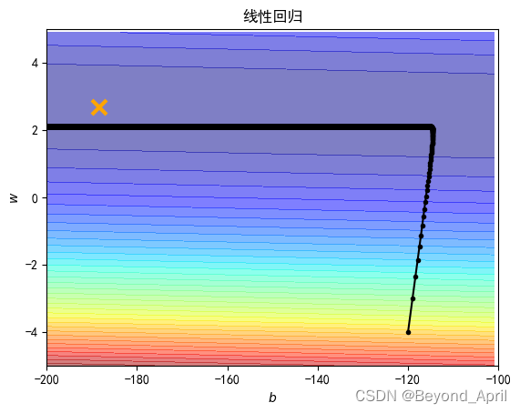
# plot the figure
plt.contourf(x, y, Z, 50, alpha=0.5, cmap=plt.get_cmap('jet'))  # 填充等高线
plt.plot([-188.4], [2.67], 'x', ms=12, mew=3, color="orange")
plt.plot(b_history, w_history, 'o-', ms=3, lw=1.5, color='black')
plt.xlim(-200, -100)
plt.ylim(-5, 5)
plt.xlabel(r'$b$')
plt.ylabel(r'$w$')
plt.title("线性回归")
plt.show()
三、参考文档
来自Datawhale的投喂
李宏毅《机器学习》开源内容1:
https://linklearner.com/datawhale-homepage/#/learn/detail/93
李宏毅《机器学习》开源内容2:
https://github.com/datawhalechina/leeml-notes
李宏毅《机器学习》开源内容3:
https://gitee.com/datawhalechina/leeml-notes
来自官方的投喂
李宏毅《机器学习》官方地址
http://speech.ee.ntu.edu.tw/~tlkagk/courses.html
李沐《动手学深度学习》官方地址
https://zh-v2.d2l.ai/
来自广大网友的投喂
numpy.array()与numpy.sarray()的区别
看这里
numpy.meshgrid()的详细解读
https://blog.csdn.net/lllxxq141592654/article/details/81532855
总结
本节内容是后面所有内容的基础,其实还有很多需要拓展深入的内容,本篇结束还没有把更多的内容总结出来,陆续整理好,希望尽早和大家见面,感谢Datawhale的小伙伴特别是组内的小伙伴们,大家加油!
- 模型假设;模型评估;最佳模型
- 模型验证
- 模型优化