决策树生成、决策树可视化、决策树算法api、泰坦尼克号乘客生存预测案例代码

一、决策树算法api

class sklearn.tree.DecisionTreeClassifier(criterion=’gini’,max_depth=None,random_state=None)
- criterion：特征选择标准，"gini"或者"entropy"，前者代表基尼系数，后者代表信息增益，默认"gini"，即CART算法
- min_samples_split：内部节点再划分所需最小样本数，这个值限制了子树继续划分的条件，如果某节点的样本数少于min_samples_split，则不会继续再尝试选择最优特征来进行划分。默认是2，如果样本量不大，不需要管这个值。如果样本量数量级非常大，则推荐增大这个值，10万样本建立决策树时可参考选择min_samples_split=10
- min_samples_leaf：叶子节点最少样本数，这个值限制了叶子节点最少的样本数，如果某叶子节点数目小于样本数，则会和兄弟节点一起被剪枝。默认是1，可以输入最少的样本数的整数，或者最少样本数占样本总数的百分比。如果样本量不大，不需要管这个值。如果样本量数量级非常大，则推荐增大这个值。10万样本可参考选择min_samples_leaf=5
- max_depth：决策树最大深度，决策树的最大深度，默认可以不输入，如果不输入的话，决策树在建立子树的时候不会限制子树的深度。一般来说，数据少或者特征少的时候可以不管这个值。如果模型样本量多，特征也多的情况下，推荐限制这个最大深度，具体的取值取决于数据的分布。常用的可以取值10-100之间
- random_state：随机数种子

二、案例：泰坦尼克号乘客生存预测

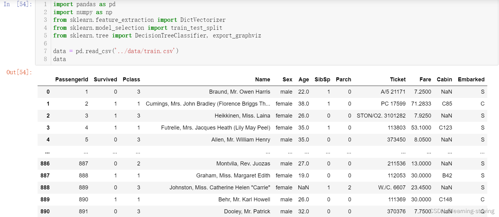
泰坦尼克号数据：在泰坦尼克号和titanic2数据帧描述泰坦尼克号上的个别乘客的生存状态，这里使用的数据集是由各种研究人员开始的，其中包括许多研究人员创建的旅客名单，由Michael A. Findlay编辑，提取的数据集中的特征是票的类别、存活、姓名、性别、年龄等

泰坦尼克号训练数据train.csv内容及使用过程如下

完整代码如下

import pandas as pd
import numpy as np
from sklearn.feature_extraction import DictVectorizer
from sklearn.model_selection import train_test_split
from sklearn.tree import DecisionTreeClassifier, export_graphviz

data = pd.read_csv('../data/train.csv')
data
------------------------------------------
data.describe()
------------------------
# 数据基本处理,确定特征值、目标值
x = data[["Pclass", "Age", "Sex"]]
x
------------------------
y = data["Survived"]
y.head()
------------------------
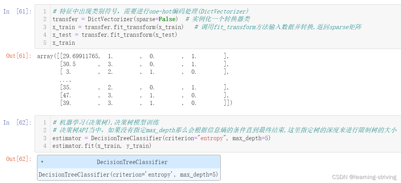
# 缺失值需要处理，将特征当中有类别的这些特征进行字典特征抽取
x['Age'].fillna(value=x['Age'].mean(), inplace=True)
x
-------------------------------------------
# 数据集划分
x_train, x_test, y_train, y_test = train_test_split(x, y, random_state=22, test_size=0.2)
x.head()
-------------------------------------------
# 特征工程(字典特征抽取)
# x.to_dict(orient="records") 需要将数组特征转换成字典数据
x_train = x_train.to_dict(orient="records")
x_test = x_test.to_dict(orient="records")
x_train
-------------------------------------------
# 特征中出现类别符号，需要进行one-hot编码处理(DictVectorizer)
transfer = DictVectorizer(sparse=False)  # 实例化一个转换器类
x_train = transfer.fit_transform(x_train)   # 调用fit_transform方法输入数据并转换,返回sparse矩阵
x_test = transfer.fit_transform(x_test)
x_train
-------------------------------------------
# 机器学习(决策树),决策树模型训练
# 决策树API当中，如果没有指定max_depth那么会根据信息熵的条件直到最终结束,这里指定树的深度来进行限制树的大小
estimator = DecisionTreeClassifier(criterion="entropy", max_depth=5)
estimator.fit(x_train, y_train)
-------------------------------------------
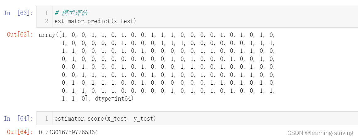
# 模型评估
estimator.predict(x_test)  # 预测值
-------------------------
estimator.score(x_test, y_test)   # 准确率

三、决策树可视化

保存树的结构到dot文件

sklearn.tree.export_graphviz()：该函数能够导出DOT格式
- tree.export_graphviz(estimator,out_file='tree.dot’,feature_names=[‘’,’’])
优点：简单的理解和解释，树木可视化
缺点：决策树学习者可以创建不能很好地推广数据的过于复杂的树，容易发生过拟合
改进：
- 减枝cart算法
- 随机森林（集成学习的一种）

企业重要决策，由于决策树很好的分析能力，在决策过程应用较多，可以选择特征

在前面代码基础上继续执行以下代码

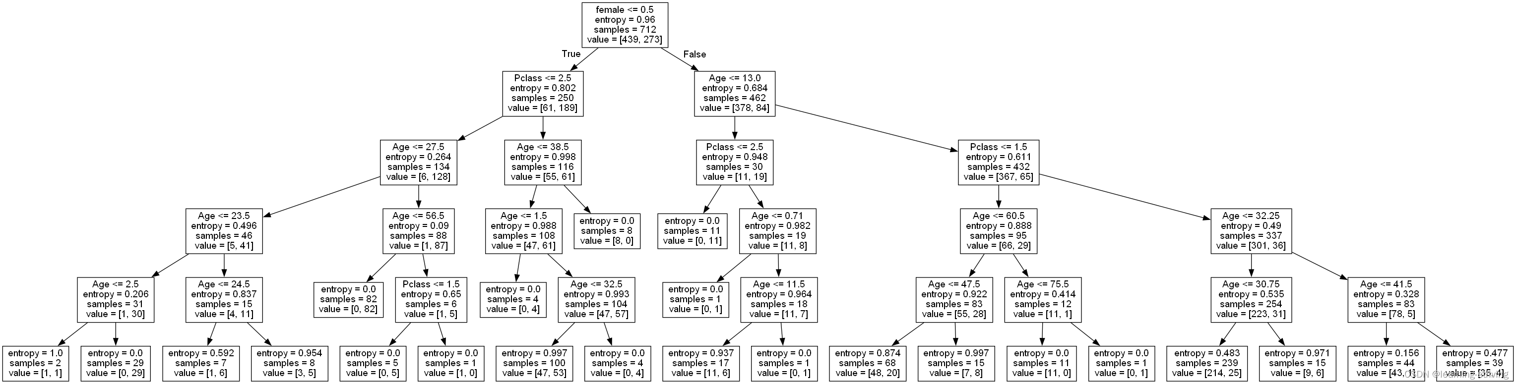
export_graphviz(estimator, out_file="../data/tree.dot", feature_names=['Age', 'Pclass', 'male', 'female'])

如下，将在data目录下生成tree.dot文件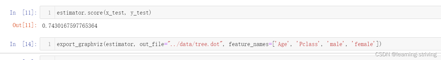

tree.dot文件内容如下

digraph Tree {
node [shape=box, fontname="helvetica"] ;
edge [fontname="helvetica"] ;
0 [label="female <= 0.5\nentropy = 0.96\nsamples = 712\nvalue = [439, 273]"] ;
1 [label="Pclass <= 2.5\nentropy = 0.802\nsamples = 250\nvalue = [61, 189]"] ;
0 -> 1 [labeldistance=2.5, labelangle=45, headlabel="True"] ;
2 [label="Age <= 27.5\nentropy = 0.264\nsamples = 134\nvalue = [6, 128]"] ;
1 -> 2 ;
3 [label="Age <= 23.5\nentropy = 0.496\nsamples = 46\nvalue = [5, 41]"] ;
2 -> 3 ;
4 [label="Age <= 2.5\nentropy = 0.206\nsamples = 31\nvalue = [1, 30]"] ;
3 -> 4 ;
5 [label="entropy = 1.0\nsamples = 2\nvalue = [1, 1]"] ;
4 -> 5 ;
6 [label="entropy = 0.0\nsamples = 29\nvalue = [0, 29]"] ;
4 -> 6 ;
7 [label="Age <= 24.5\nentropy = 0.837\nsamples = 15\nvalue = [4, 11]"] ;
3 -> 7 ;
8 [label="entropy = 0.592\nsamples = 7\nvalue = [1, 6]"] ;
7 -> 8 ;
9 [label="entropy = 0.954\nsamples = 8\nvalue = [3, 5]"] ;
7 -> 9 ;
10 [label="Age <= 56.5\nentropy = 0.09\nsamples = 88\nvalue = [1, 87]"] ;
2 -> 10 ;
11 [label="entropy = 0.0\nsamples = 82\nvalue = [0, 82]"] ;
10 -> 11 ;
12 [label="Pclass <= 1.5\nentropy = 0.65\nsamples = 6\nvalue = [1, 5]"] ;
10 -> 12 ;
13 [label="entropy = 0.0\nsamples = 5\nvalue = [0, 5]"] ;
12 -> 13 ;
14 [label="entropy = 0.0\nsamples = 1\nvalue = [1, 0]"] ;
12 -> 14 ;
15 [label="Age <= 38.5\nentropy = 0.998\nsamples = 116\nvalue = [55, 61]"] ;
1 -> 15 ;
16 [label="Age <= 1.5\nentropy = 0.988\nsamples = 108\nvalue = [47, 61]"] ;
15 -> 16 ;
17 [label="entropy = 0.0\nsamples = 4\nvalue = [0, 4]"] ;
16 -> 17 ;
18 [label="Age <= 32.5\nentropy = 0.993\nsamples = 104\nvalue = [47, 57]"] ;
16 -> 18 ;
19 [label="entropy = 0.997\nsamples = 100\nvalue = [47, 53]"] ;
18 -> 19 ;
20 [label="entropy = 0.0\nsamples = 4\nvalue = [0, 4]"] ;
18 -> 20 ;
21 [label="entropy = 0.0\nsamples = 8\nvalue = [8, 0]"] ;
15 -> 21 ;
22 [label="Age <= 13.0\nentropy = 0.684\nsamples = 462\nvalue = [378, 84]"] ;
0 -> 22 [labeldistance=2.5, labelangle=-45, headlabel="False"] ;
23 [label="Pclass <= 2.5\nentropy = 0.948\nsamples = 30\nvalue = [11, 19]"] ;
22 -> 23 ;
24 [label="entropy = 0.0\nsamples = 11\nvalue = [0, 11]"] ;
23 -> 24 ;
25 [label="Age <= 0.71\nentropy = 0.982\nsamples = 19\nvalue = [11, 8]"] ;
23 -> 25 ;
26 [label="entropy = 0.0\nsamples = 1\nvalue = [0, 1]"] ;
25 -> 26 ;
27 [label="Age <= 11.5\nentropy = 0.964\nsamples = 18\nvalue = [11, 7]"] ;
25 -> 27 ;
28 [label="entropy = 0.937\nsamples = 17\nvalue = [11, 6]"] ;
27 -> 28 ;
29 [label="entropy = 0.0\nsamples = 1\nvalue = [0, 1]"] ;
27 -> 29 ;
30 [label="Pclass <= 1.5\nentropy = 0.611\nsamples = 432\nvalue = [367, 65]"] ;
22 -> 30 ;
31 [label="Age <= 60.5\nentropy = 0.888\nsamples = 95\nvalue = [66, 29]"] ;
30 -> 31 ;
32 [label="Age <= 47.5\nentropy = 0.922\nsamples = 83\nvalue = [55, 28]"] ;
31 -> 32 ;
33 [label="entropy = 0.874\nsamples = 68\nvalue = [48, 20]"] ;
32 -> 33 ;
34 [label="entropy = 0.997\nsamples = 15\nvalue = [7, 8]"] ;
32 -> 34 ;
35 [label="Age <= 75.5\nentropy = 0.414\nsamples = 12\nvalue = [11, 1]"] ;
31 -> 35 ;
36 [label="entropy = 0.0\nsamples = 11\nvalue = [11, 0]"] ;
35 -> 36 ;
37 [label="entropy = 0.0\nsamples = 1\nvalue = [0, 1]"] ;
35 -> 37 ;
38 [label="Age <= 32.25\nentropy = 0.49\nsamples = 337\nvalue = [301, 36]"] ;
30 -> 38 ;
39 [label="Age <= 30.75\nentropy = 0.535\nsamples = 254\nvalue = [223, 31]"] ;
38 -> 39 ;
40 [label="entropy = 0.483\nsamples = 239\nvalue = [214, 25]"] ;
39 -> 40 ;
41 [label="entropy = 0.971\nsamples = 15\nvalue = [9, 6]"] ;
39 -> 41 ;
42 [label="Age <= 41.5\nentropy = 0.328\nsamples = 83\nvalue = [78, 5]"] ;
38 -> 42 ;
43 [label="entropy = 0.156\nsamples = 44\nvalue = [43, 1]"] ;
42 -> 43 ;
44 [label="entropy = 0.477\nsamples = 39\nvalue = [35, 4]"] ;
42 -> 44 ;
}

可将tree.dot文件中内容复制到Webgraphviz网站中执行，以实现决策树可视化，本人运行时该网站好像失效了，加载不出，如下

改用以下方式执行，见：graphviz安装及使用、决策树生成

生成决策树如下

学习导航：http://xqnav.top/

决策树生成、决策树可视化、决策树算法api、泰坦尼克号乘客生存预测案例代码

一、决策树算法api

二、案例：泰坦尼克号乘客生存预测

三、决策树可视化

猜你喜欢