前导
更多文章代码详情可查看博主个人网站:https://www.iwtmbtly.com/
导入需要使用的库和文件:
>>> import pandas as pd
>>> import numpy as np
>>> df = pd.read_csv('data/table_missing.csv')
>>> df.head()
  School Class      ID Gender   Address  Height  Weight  Math Physics
0    S_1   C_1     NaN      M  street_1     173     NaN  34.0      A+
1    S_1   C_1     NaN      F  street_2     192     NaN  32.5      B+
2    S_1   C_1  1103.0      M  street_2     186     NaN  87.2      B+
3    S_1   NaN     NaN      F  street_2     167    81.0  80.4     NaN
4    S_1   C_1  1105.0    NaN  street_4     159    64.0  84.8      A-
在接下来的学习中,会接触到数据预处理中比较麻烦的类型,即缺失数据和文本数据(尤其是混杂型文本)
Pandas在步入1.0后,对数据类型也做出了新的尝试,尤其是Nullable类型和String类型,了解这些可能在未来成为主流的新特性是必要的
一、缺失观测及其类型
(一)了解缺失信息
1. isna和notna方法
对Series使用会返回布尔列表
>>> df['Physics'].isna().head()
0    False
1    False
2    False
3     True
4    False
Name: Physics, dtype: bool
>>> df['Physics'].notna().head()
0     True
1     True
2     True
3    False
4     True
Name: Physics, dtype: bool
对DataFrame使用会返回布尔表
>>> df.isna().head()
   School  Class     ID  Gender  Address  Height  Weight   Math  Physics
0   False  False   True   False    False   False    True  False    False
1   False  False   True   False    False   False    True  False    False
2   False  False  False   False    False   False    True  False    False
3   False   True   True   False    False   False   False  False     True
4   False  False  False    True    False   False   False  False    False
但对于DataFrame我们更关心到底每列有多少缺失值
>>> df.isna().sum()
School      0
Class       4
ID          6
Gender      7
Address     0
Height      0
Weight     13
Math        5
Physics     4
dtype: int64
此外,可以通过第1章中介绍的info函数查看缺失信息
>>> df.info()
<class 'pandas.core.frame.DataFrame'>
Data columns (total 9 columns):
 #   Column   Non-Null Count  Dtype
---  ------   --------------  -----
 0   School   35 non-null     object
 1   Class    31 non-null     object
 2   ID       29 non-null     float64
 3   Gender   28 non-null     object
 4   Address  35 non-null     object
 5   Height   35 non-null     int64
 6   Weight   22 non-null     float64
 7   Math     30 non-null     float64
 8   Physics  31 non-null     object
dtypes: float64(3), int64(1), object(5)
2. 查看缺失值的所以在行
以最后一列为例,挑出该列缺失值的行:
>>> df[df['Physics'].isna()]
   School Class      ID Gender   Address  Height  Weight  Math Physics
3     S_1   NaN     NaN      F  street_2     167    81.0  80.4     NaN
8     S_1   C_2  1204.0      F  street_5     162    63.0  33.8     NaN
13    S_1   C_3  1304.0    NaN  street_2     195    70.0  85.2     NaN
22    S_2   C_2  2203.0      M  street_4     155    91.0  73.8     NaN
3. 挑选出所有非缺失值列
使用all就是全部非缺失值,如果是any就是至少有一个不是缺失值:
>>> df[df.notna().all(1)]
   School Class      ID Gender   Address  Height  Weight  Math Physics
5     S_1   C_2  1201.0      M  street_5     159    68.0  97.0      A-
6     S_1   C_2  1202.0      F  street_4     176    94.0  63.5      B-
12    S_1   C_3  1303.0      M  street_7     188    82.0  49.7       B
17    S_2   C_1  2103.0      M  street_4     157    61.0  52.5      B-
21    S_2   C_2  2202.0      F  street_7     194    77.0  68.5      B+
25    S_2   C_3  2301.0      F  street_4     157    78.0  72.3      B+
27    S_2   C_3  2303.0      F  street_7     190    99.0  65.9       C
28    S_2   C_3  2304.0      F  street_6     164    81.0  95.5      A-
29    S_2   C_3  2305.0      M  street_4     187    73.0  48.9       B
(二)三种缺失符号
1. np.nan
np.nan是一个麻烦的东西,首先它不等与任何东西,甚至不等于自己:
>>> np.nan == np.nan
False
>>> np.nan == 0
False
>>> np.nan == None
False
在用equals函数比较时,自动略过两侧全是np.nan的单元格,因此结果不会影响
>>> df.equals(df)
True
其次,它在numpy中的类型为浮点,由此导致数据集读入时,即使原来是整数的列,只要有缺失值就会变为浮点型:
>>> type(np.nan)
<class 'float'>
>>> pd.Series([1,2,3]).dtype
dtype('int64')
>>> pd.Series([1,np.nan,3]).dtype
dtype('float64')
此外,对于布尔类型的列表,如果是np.nan填充,那么它的值会自动变为True而不是False:
>>> pd.Series([1,np.nan,3],dtype='bool')
0    True
1    True
2    True
dtype: bool
但当修改一个布尔列表时,会改变列表类型,而不是赋值为True:
>>> s = pd.Series([True, False], dtype='bool')
>>> s[1] = np.nan
>>> s
0    True
1     NaN
dtype: object
在所有的表格读取后,无论列是存放什么类型的数据,默认的缺失值全为np.nan类型
因此整型列转为浮点;而字符由于无法转化为浮点,因此只能归并为object类型(‘O’),原来是浮点型的则类型不变:
>>> df['ID'].dtype
dtype('float64')
>>> df['Math'].dtype
dtype('float64')
>>> df['Class'].dtype
dtype('O')
2. None
None比前者稍微好些,至少它会等于自身:
>>> None == None
True
>>> None is None
True
它的布尔值为False:
>>> pd.Series([None], dtype='bool')
0    False
dtype: bool
修改布尔列表不会改变数据类型:
>>> s = pd.Series([True,False],dtype='bool')
>>> s[0]=None
>>> s
0      NaN
1    False
dtype: object
s = pd.Series([1,0],dtype='bool')
s[0]=None
s
在传入数值类型后,会自动变为np.nan,只有当传入object类型是保持不动,几乎可以认为,除非人工命名None,它基本不会自动出现在Pandas中:
>>> type(pd.Series([1,None])[1])
<class 'numpy.float64'>
>>> type(pd.Series([1,None],dtype='O')[1])
<class 'NoneType'>
在使用equals函数时不会被略过,因此下面的情况下返回False:
>>> pd.Series([None]).equals(pd.Series([np.nan]))
False
3. NaT
NaT是针对时间序列的缺失值,是Pandas的内置类型,可以完全看做时序版本的np.nan,与自己不等,且使用equals时也会被跳过
>>> s_time = pd.Series([pd.Timestamp('20120101')]*5)
>>> s_time
0   2012-01-01
1   2012-01-01
4   2012-01-01
dtype: datetime64[ns]
>>> s_time[2] = None
>>> s_time
0   2012-01-01
1   2012-01-01
3   2012-01-01
dtype: datetime64[ns]
>>> s_time
3   2012-01-01
4   2012-01-01
dtype: datetime64[ns]
>>> s_time
0   2012-01-01
1   2012-01-01
2          NaT
3   2012-01-01
4   2012-01-01
dtype: datetime64[ns]
>>> type(s_time[2])
<class 'pandas._libs.tslibs.nattype.NaTType'>
>>> s_time[2] == s_time[2]
False
>>> s_time.equals(s_time)
True
>>> s = pd.Series([True,False],dtype='bool')
>>> s[1]=pd.NaT
>>> s
0    True
1     NaT
dtype: object
(三)Nullable类型与NA符号
这是Pandas在1.0新版本中引入的重大改变,其目的就是为了(在若干版本后)解决之前出现的混乱局面,统一缺失值处理方法
“The goal of pd.NA is provide a “missing” indicator that can be used consistently across data types (instead of np.nan, None or pd.NaT depending on the data type).”——User Guide for Pandas v-1.0
官方鼓励用户使用新的数据类型和缺失类型pd.NA
1. Nullable整形
对于该种类型而言,它与原来标记int上的符号区别在于首字母大写:‘Int’:
>>> s_original = pd.Series([1, 2], dtype="int64")
>>> s_original
0    1
1    2
dtype: int64
>>> s_new = pd.Series([1, 2], dtype="Int64")
>>> s_new
0    1
1    2
dtype: Int64
它的好处就在于,其中前面提到的三种缺失值都会被替换为统一的NA符号,且不改变数据类型:
>>> s_original
0    1.0
1    NaN
dtype: float64
>>> s_new[1] = np.nan
>>> s_new
0       1
1    <NA>
dtype: Int64
>>> s_new[1] = None
>>> s_new
0       1
1    <NA>
dtype: Int64
>>> s_new[1] = pd.NaT
>>> s_new
0       1
1    <NA>
dtype: Int64
2. Nullable布尔
对于该种类型而言,作用与上面的类似,记号为boolean
>>> s_original = pd.Series([1, 0], dtype="bool")
1    False
dtype: bool
>>> s_new = pd.Series([0, 1], dtype="boolean")
1     True
dtype: boolean
>>> s_original[0] = np.nan
1    False
dtype: object
>>> s_original = pd.Series([1, 0], dtype="bool")  # 此处重新加一句是因为前面赋值改变了bool类型
>>> s_original
0      NaN
1    False
dtype: object
>>> s_new[0] = np.nan
>>> s_new
0    <NA>
1    True
dtype: boolean
>>> s_new[0] = None
>>> s_new
0    <NA>
1    True
dtype: boolean
>>> s_new[0] = pd.NaT
>>> s_new
0    <NA>
1    True
dtype: boolean
需要注意的是,含有pd.NA的布尔列表在1.0.2之前的版本作为索引时会报错,这是一个之前的bug,现已经修复
>>> s = pd.Series(['dog','cat'])
>>> s[s_new]
1    cat
dtype: object
3. string类型
该类型是1.0的一大创新,目的之一就是为了区分开原本含糊不清的object类型,这里将简要地提及string。
它本质上也属于Nullable类型,因为并不会因为含有缺失而改变类型:
>>> s = pd.Series(['dog','cat'],dtype='string')
>>> s
0    dog
1    cat
dtype: string
>>> s[0] = np.nan
>>> s
0    <NA>
1     cat
dtype: string
>>> s[0] = None
>>> s
0    <NA>
1     cat
dtype: string
>>> s[0] = pd.NaT
>>> s
0    <NA>
1     cat
dtype: string
此外,和object类型的一点重要区别就在于,在调用字符方法后,string类型返回的是Nullable类型,object则会根据缺失类型和数据类型而改变
>>> s = pd.Series(["a", None, "b"], dtype="string")
>>> s.str.count('a')
1    <NA>
2       0
dtype: Int64
>>> s2 = pd.Series(["a", None, "b"], dtype="object")
>>> s2.str.count("a")
0    1.0
1    NaN
2    0.0
dtype: float64
>>> s.str.isdigit()
0    False
1     <NA>
2    False
dtype: boolean
>>> s2.str.isdigit()
0    False
1     None
2    False
dtype: object
(四)NA的特性
1. 逻辑运算
只需看该逻辑运算的结果是否依赖pd.NA的取值,如果依赖,则结果还是NA,如果不依赖,则直接计算结果:
>>> True | pd.NA
True
>>> pd.NA | True
True
>>> False | pd.NA
<NA>
>>> False & pd.NA
False
>>> True & pd.NA
<NA>
取值不明直接报错
>>> bool(pd.NA)
Traceback (most recent call last):
  File "<stdin>", line 1, in <module>
  File "pandas\_libs\missing.pyx", line 446, in pandas._libs.missing.NAType.__bool__
TypeError: boolean value of NA is ambiguous
2. 算术运算和比较运算
这里只需记住除了下面两类情况,其他结果都是NA即可:
>>> pd.NA ** 0
1
>>> 1 ** pd.NA
1
其他情况:
>>> pd.NA + 1
<NA>
>>> "a" * pd.NA
<NA>
>>> pd.NA == pd.NA
<NA>
>>> pd.NA < 2.5
<NA>
>>> np.log(pd.NA)
<NA>
>>> np.add(pd.NA, 1)
<NA>
(五)convert_dtypes方法
这个函数的功能往往就是在读取数据时,就把数据列转为Nullable类型,是1.0的新函数:
>>> pd.read_csv('data/table_missing.csv').dtypes
School      object
ID         float64
Gender      object
Address     object
Height       int64
Weight     float64
Math       float64
Physics     object
dtype: object
>>> pd.read_csv('data/table_missing.csv').convert_dtypes().dtypes
School      string
Class       string
ID           Int64
Gender      string
Address     string
Height       Int64
Weight       Int64
Math       Float64
Physics     string
dtype: object
二、缺失数据的运算与分组
(一)加号与乘号规则
使用加法时,缺失值为0:
>>> s = pd.Series([2,3,np.nan,4])
>>> s.sum()
9.0
使用乘法时,缺失值为1:
>>> s.prod()
24.0
使用累计函数时,缺失值自动略过:
>>> s.cumsum()	# 累加
0    2.0
1    5.0
2    NaN
3    9.0
dtype: float64

>>> s.cumprod()	# 累乘
0     2.0
1     6.0
2     NaN
3    24.0
dtype: float64

>>> s.pct_change()
0         NaN
1    0.500000
2    0.000000
3    0.333333
dtype: float64
(二)groupby方法中的缺失值
自动忽略为缺失值的组:
>>> df_g = pd.DataFrame({

    'one':['A','B','C','D',np.nan],'two':np.random.randn(5)})
>>> df_g
   one       two
0    A -1.507732
1    B -0.290983
2    C  0.301578
3    D  1.186912
4  NaN  0.369869

>>> df_g.groupby('one').groups
{

    'A': Int64Index([0], dtype='int64'),
 'B': Int64Index([1], dtype='int64'),
 'C': Int64Index([2], dtype='int64'),
 'D': Int64Index([3], dtype='int64')}
三、填充与剔除
(一)fillna方法
1. 值填充与前后向填充(分别与ffill方法和bfill方法等价)
>>> df['Physics'].fillna('missing').head()
1         B+
2         B+
3    missing
4         A-
Name: Physics, dtype: object
>>> df['Physics'].fillna(method='ffill').head()
0    A+
1    B+
2    B+
3    B+
4    A-
Name: Physics, dtype: object
>>> df['Physics'].fillna(method='backfill').head()
0    A+
1    B+
2    B+
3    A-
4    A-
Name: Physics, dtype: object
2. 填充中的对齐特性
>>> df_f = pd.DataFrame({

    'A':[1,3,np.nan],'B':[2,4,np.nan],'C':[3,5,np.nan]})
>>> df_f.fillna(df_f.mean())
     A    B    C
0  1.0  2.0  3.0
1  3.0  4.0  5.0
2  2.0  3.0  4.0
返回的结果中没有C,根据对齐特点不会被填充:
>>> df_f.fillna(df_f.mean()[['A','B']])
     A    B    C
0  1.0  2.0  3.0
1  3.0  4.0  5.0
2  2.0  3.0  NaN
(二)dropna方法
1. axis参数
>>> df_d = pd.DataFrame({

    'A':[np.nan,np.nan,np.nan],'B':[np.nan,3,2],'C':[3,2,1]})
>>> df_d
    A    B  C
0 NaN  NaN  3
1 NaN  3.0  2
2 NaN  2.0  1
>>> df_d.dropna(axis=0)
Empty DataFrame
Columns: [A, B, C]
Index: []
>>> df_d.dropna(axis=1)
   C
0  3
1  2
2  1
2. how参数(可以选all或者any,表示全为缺失去除和存在缺失去除)
>>> df_d.dropna(axis=1,how='all')
     B  C
0  NaN  3
1  3.0  2
2  2.0  1
>>> df_d.dropna(axis=1,how='any')
   C
0  3
1  2
2  1
3. subset参数(即在某一组列范围中搜索缺失值)
>>> df_d.dropna(axis=0,subset=['B','C'])
    A    B  C
1 NaN  3.0  2
2 NaN  2.0  1
四、插值(interpolation)
(一)线性插值
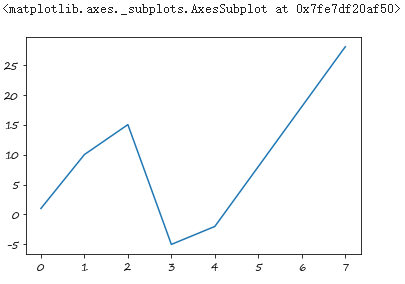
1. 索引无关的线性插值
默认状态下,interpolate会对缺失的值进行线性插值:
>>> s = pd.Series([1,10,15,-5,-2,np.nan,np.nan,28])
0     1.0
2    15.0
3    -5.0
4    -2.0
5     NaN
6     NaN
7    28.0
dtype: float64
>>> s.interpolate()
0     1.0
1    10.0
2    15.0
3    -5.0
4    -2.0
5     8.0
6    18.0
7    28.0
dtype: float64
>>> s.interpolate().plot()
<matplotlib.axes._subplots.AxesSubplot at 0x7fe7df20af50>
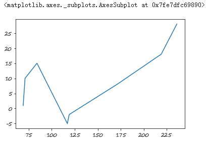
此时的插值与索引无关:
>>> s.index = np.sort(np.random.randint(50,300,8))
>>> s.interpolate()	# 值不变
56      1.0
112    10.0
134    15.0
144    -5.0
164    -2.0
254     8.0
265    18.0
267    28.0
dtype: float64
>>> s.interpolate().plot()	# #后面三个点不是线性的
<matplotlib.axes._subplots.AxesSubplot at 0x7fe7dfc69890>
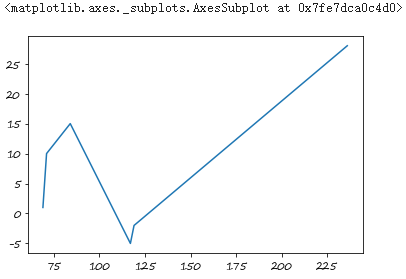
2. 与索引有关的插值
method中的index和time选项可以使插值线性地依赖索引,即插值为索引的线性函数:
>>> s.interpolate(method='index').plot()	# 可以看到与上面的区别
<matplotlib.axes._subplots.AxesSubplot at 0x7fe7dca0c4d0>
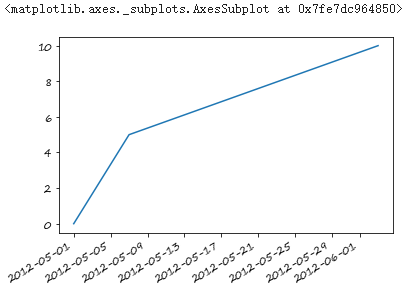
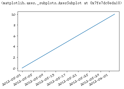
如果索引是时间,那么可以按照时间长短插值:
>>> s_t = pd.Series([0,np.nan,10]
...         ,index=[pd.Timestamp('2012-05-01'),pd.Timestamp('2012-05-07'),pd.Timestamp('2012-06-03')])
>>> s_t
2012-05-01     0.0
2012-05-07     NaN
2012-06-03    10.0
dtype: float64
>>> s_t.interpolate().plot()
<matplotlib.axes._subplots.AxesSubplot at 0x7fe7dc964850>
>>> s_t.interpolate(method='time').plot()
<matplotlib.axes._subplots.AxesSubplot at 0x7fe7dc8eda10>
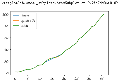
(二)高级插值方法
此处的高级指的是与线性插值相比较,例如样条插值、多项式插值、阿基玛插值等(需要安装Scipy),方法详情请看这里
关于这部分仅给出一个官方的例子,因为插值方法是数值分析的内容,而不是Pandas中的基本知识:
>>> ser = pd.Series(np.arange(1, 10.1, .25) ** 2 + np.random.randn(37))
>>> missing = np.array([4, 13, 14, 15, 16, 17, 18, 20, 29])
>>> ser[missing] = np.nan
>>> methods = ['linear', 'quadratic', 'cubic']
>>> df = pd.DataFrame({

    m: ser.interpolate(method=m) for m in methods})
>>> df.plot()
<matplotlib.axes._subplots.AxesSubplot at 0x7fe7dc86f810>
(三)interpolate中的限制参数
1. limit表示最多插入多少个
>>> s = pd.Series([1,np.nan,np.nan,np.nan,5])
>>> s.interpolate(limit=2)
0    1.0
1    2.0
2    3.0
3    NaN
4    5.0
dtype: float64
2. limit_direction表示插值方向,可选forward,backward,both,默认前向
>>> s = pd.Series([np.nan,np.nan,1,np.nan,np.nan,np.nan,5,np.nan,np.nan,])
>>> s.interpolate(limit_direction='backward')
0    1.0
1    1.0
2    1.0
4    3.0
5    4.0
6    5.0
7    NaN
8    NaN
dtype: float64
3. limit_area表示插值区域,可选inside,outside,默认None
>>> s = pd.Series([np.nan,np.nan,1,np.nan,np.nan,np.nan,5,np.nan,np.nan,])
>>> s.interpolate(limit_area='inside')
0    NaN
1    NaN
2    1.0
3    2.0
4    3.0
5    4.0
6    5.0
7    NaN
8    NaN
dtype: float64
>>> s = pd.Series([np.nan,np.nan,1,np.nan,np.nan,np.nan,5,np.nan,np.nan,])
>>> s.interpolate(limit_area='outside')
0    NaN
1    NaN
2    1.0
3    NaN
4    NaN
5    NaN
6    5.0
7    5.0
8    5.0
dtype: float64