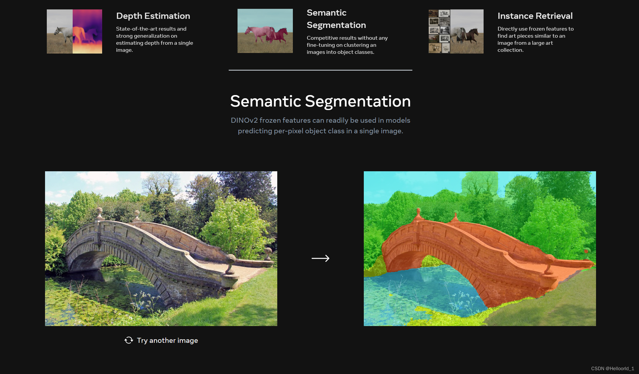
meta的dinov2的发布;无需文字标签,完全自监督的Meta视觉大模型!
示例如下:
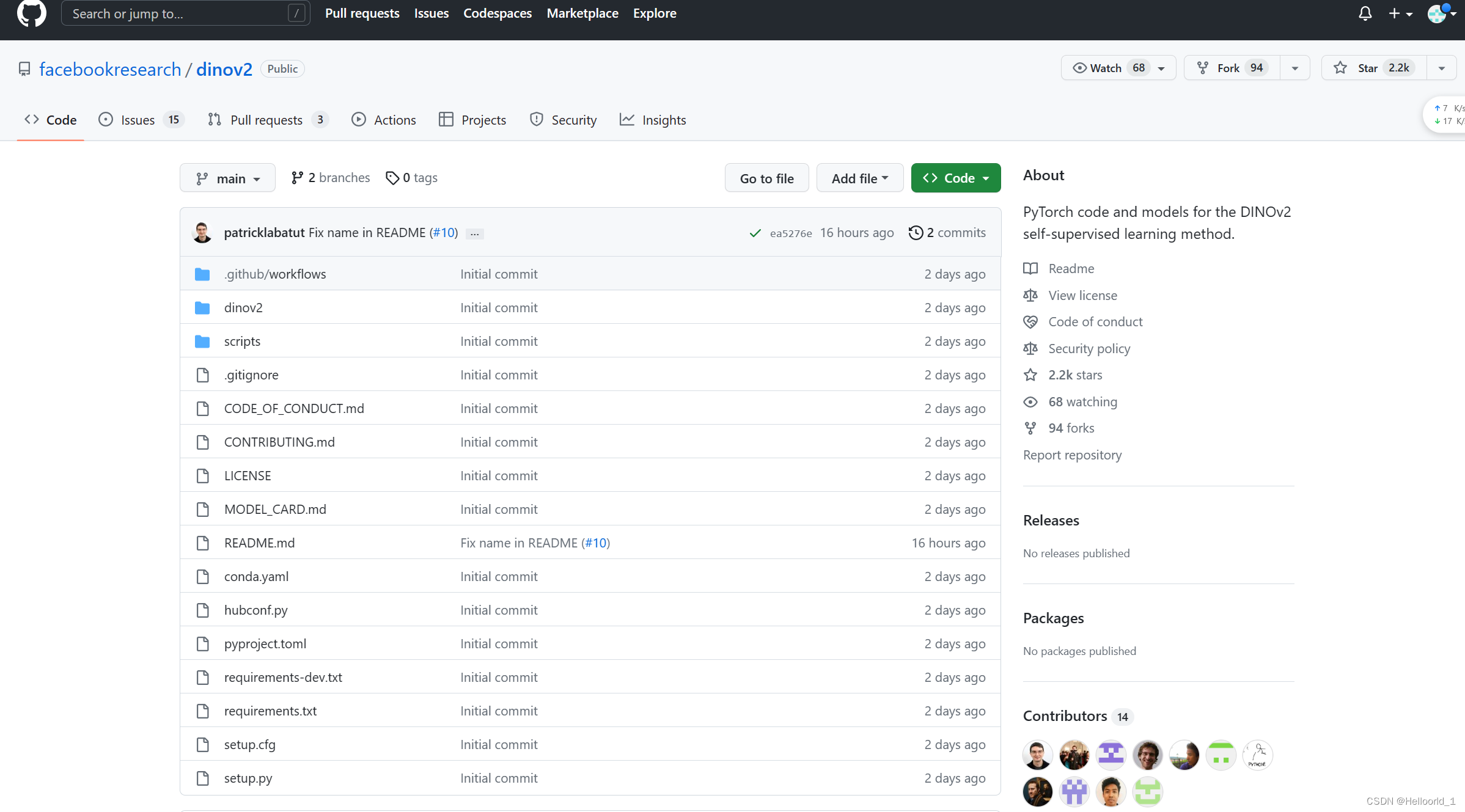
部署到本地的方法
先下载code ->zip
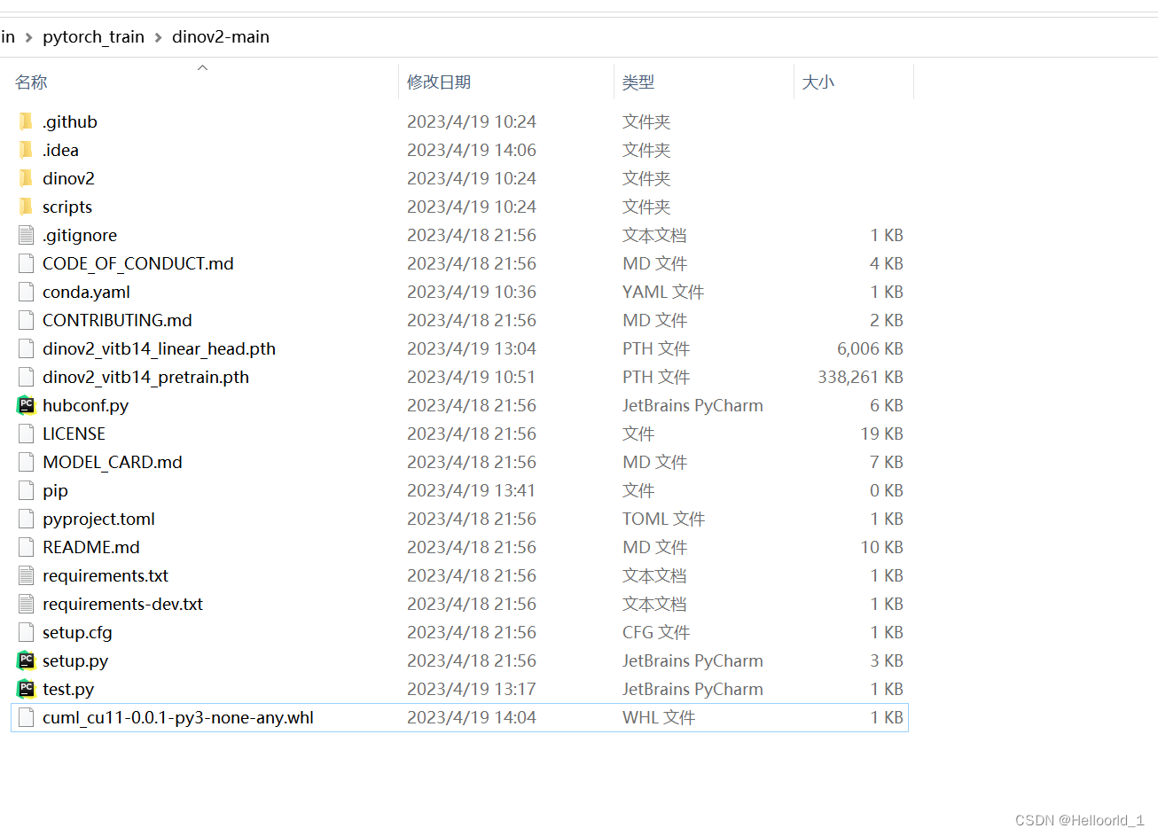
然后解压到文件夹如下:
配置环境命令(本文只针对anconda来使用,纯python环境请自行尝试单独下载)
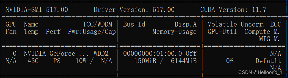
按照源码要求,需要使用11.7的CUDA,刚好我的电脑支持。
可以通过cmd输入
nvidia-smi查询支持的CUDA Version
在上述文件夹中打开cmd命令(处于当前位置),输入以下指令:
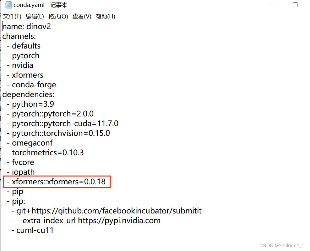
conda env create -f conda.yaml
#创建新python的环境,按照conda.yml的形式

conda activate dinov2
#激活环境
会遇到报错,用记事本打开conda.yml将红色部分先删除
再次按照上面cmd命令运行,完成后会显示done
然后手动安装剩余的包如下:
xformers-0.0.18-cp39-cp39-win_amd64.whl
submitit-1.4.5-py3-none-any.whl
cuml_cu11-0.0.1-py3-none-any.whl
包的地址可以自己下载,也可以用我提供的地址如下:
python相关补充依赖包,仅供学习交流使用!-Python文档类资源-CSDN文库
安装完成后可以查看
conda list有以下环境:
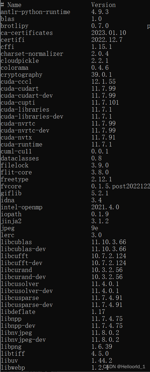
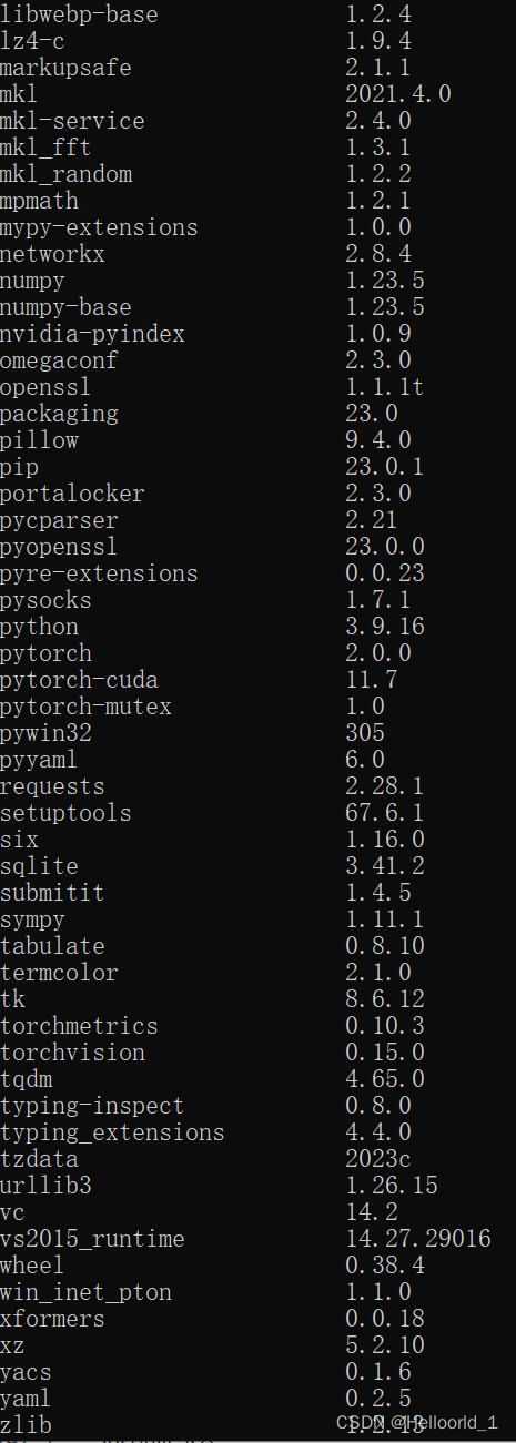
这样环境就配置完成了。
对了还需要安装sklearn
pip install scikit-learn -i https://pypi.tuna.tsinghua.edu.cn/simple然后创建一个test.py到相同解压文件目录下。
参考运行实例代码如下:
import torch
import torchvision.transforms as T
import matplotlib.pyplot as plt
from PIL import Image
from sklearn.decomposition import PCA
patch_h = 40
patch_w = 40
feat_dim = 384 # vits14
transform = T.Compose([
T.GaussianBlur(9, sigma=(0.1, 2.0)),
T.Resize((patch_h * 14, patch_w * 14)),
T.CenterCrop((patch_h * 14, patch_w * 14)),
T.ToTensor(),
T.Normalize(mean=(0.485, 0.456, 0.406), std=(0.229, 0.224, 0.225)),
])
dinov2_vitb14 = torch.hub.load('', 'dinov2_vits14',source='local').cuda()
print(dinov2_vitb14)
# extract features
features = torch.zeros(4, patch_h * patch_w, feat_dim)
imgs_tensor = torch.zeros(4, 3, patch_h * 14, patch_w * 14).cuda()
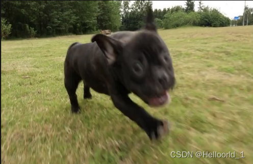
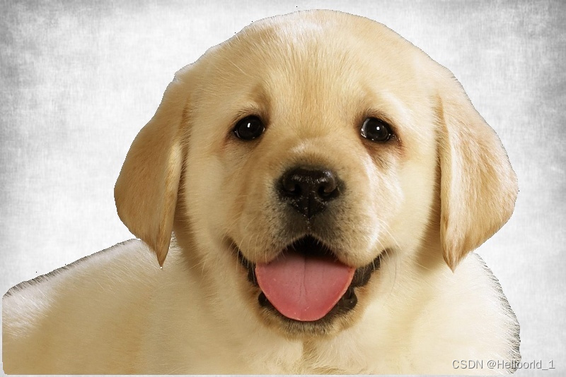
img_path = f'meta_dog.png'#输入图片路径
img = Image.open(img_path).convert('RGB')
imgs_tensor[0] = transform(img)[:3]
with torch.no_grad():
features_dict = dinov2_vitb14.forward_features(imgs_tensor)
features = features_dict['x_norm_patchtokens']
features = features.reshape(4 * patch_h * patch_w, feat_dim).cpu()
pca = PCA(n_components=3)
pca.fit(features)
pca_features = pca.transform(features)
# visualize PCA components for finding a proper threshold
plt.subplot(1, 3, 1)
plt.hist(pca_features[:, 0])
plt.subplot(1, 3, 2)
plt.hist(pca_features[:, 1])
plt.subplot(1, 3, 3)
plt.hist(pca_features[:, 2])
plt.show()
plt.close()
# uncomment below to plot the first pca component
# pca_features[:, 0] = (pca_features[:, 0] - pca_features[:, 0].min()) / (pca_features[:, 0].max() - pca_features[:, 0].min())
# for i in range(4):
# plt.subplot(2, 2, i+1)
# plt.imshow(pca_features[i * patch_h * patch_w: (i+1) * patch_h * patch_w, 0].reshape(patch_h, patch_w))
# plt.show()
# plt.close()
# segment using the first component
pca_features_bg = pca_features[:, 0] < 10
pca_features_fg = ~pca_features_bg
# plot the pca_features_bg
for i in range(4):
plt.subplot(2, 2, i+1)
plt.imshow(pca_features_bg[i * patch_h * patch_w: (i+1) * patch_h * patch_w].reshape(patch_h, patch_w))
plt.show()
# PCA for only foreground patches
pca_features_rem = pca.transform(features[pca_features_fg])
for i in range(3):
# pca_features_rem[:, i] = (pca_features_rem[:, i] - pca_features_rem[:, i].min()) / (pca_features_rem[:, i].max() - pca_features_rem[:, i].min())
# transform using mean and std, I personally found this transformation gives a better visualization
pca_features_rem[:, i] = (pca_features_rem[:, i] - pca_features_rem[:, i].mean()) / (pca_features_rem[:, i].std() ** 2) + 0.5
pca_features_rgb = pca_features.copy()
pca_features_rgb[pca_features_bg] = 0
pca_features_rgb[pca_features_fg] = pca_features_rem
pca_features_rgb = pca_features_rgb.reshape(4, patch_h, patch_w, 3)
for i in range(4):
plt.subplot(2, 2, i+1)
plt.imshow(pca_features_rgb[i][..., ::-1])
plt.savefig('features.png')#保存结果图片
plt.show()
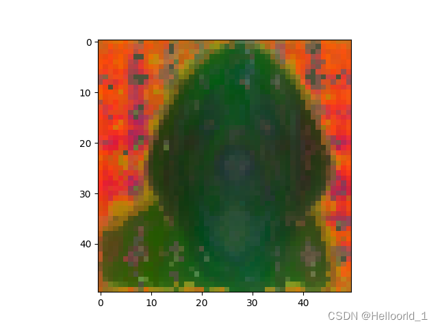
plt.close()结果如图所示:
输入图片:
输出图片:

我用的最差的vit-s模型,所以效果不太好!
5月22日
****************************新的更新**************************************************************
这里采用vit-g模型,所实现的代码和效果如下:
代码部分:
import torch

import torchvision.transforms as T

import matplotlib.pyplot as plt
import numpy as np

import matplotlib.image as mpimg

from PIL import Image

from sklearn.decomposition import PCA
import matplotlib

matplotlib.use('TkAgg')

patch_h = 50
patch_w = 50
feat_dim = 1536 # vitg14

transform = T.Compose([
    T.GaussianBlur(9, sigma=(0.1, 2.0)),
    T.Resize((patch_h * 14, patch_w * 14)),
    T.CenterCrop((patch_h * 14, patch_w * 14)),
    T.ToTensor(),
    T.Normalize(mean=(0.485, 0.456, 0.406), std=(0.229, 0.224, 0.225)),
])

dinov2_vitb14 = torch.hub.load('', 'dinov2_vitg14',source='local').cuda()

print(dinov2_vitb14)

# extract features
features = torch.zeros(4, patch_h * patch_w, feat_dim)
imgs_tensor = torch.zeros(4, 3, patch_h * 14, patch_w * 14).cuda()

img_path = f'./image/mix.jpg'#修改图片路径
img = Image.open(img_path).convert('RGB')
imgs_tensor[0] = transform(img)[:3]
with torch.no_grad():
    features_dict = dinov2_vitb14.forward_features(imgs_tensor)
    features = features_dict['x_norm_patchtokens']


features = features.reshape(4 * patch_h * patch_w, feat_dim).cpu()
print(features)
pca = PCA(n_components=3)
pca.fit(features)
pca_features = pca.transform(features)
pca_features[:, 0] = (pca_features[:, 0] - pca_features[:, 0].min()) / (pca_features[:, 0].max() - pca_features[:, 0].min())

# segment using the first component

pca_features_fg = pca_features[:, 0] >0.3
pca_features_bg = ~pca_features_fg

b=np.where(pca_features_bg)#取满足条件的下标
print("1",pca_features[:, 0])
# print(pca_features_fg)
# PCA for only foreground patches
pca.fit(features[pca_features_fg])
pca_features_rem = pca.transform(features[pca_features_fg])
for i in range(3):
    pca_features_rem[:, i] = (pca_features_rem[:, i] - pca_features_rem[:, i].min()) / (pca_features_rem[:, i].max() - pca_features_rem[:, i].min())
    # transform using mean and std, I personally found this transformation gives a better visualization
    # pca_features_rem[:, i] = (pca_features_rem[:, i] - pca_features_rem[:, i].mean()) / (pca_features_rem[:, i].std() ** 2) + 0.5

pca_features_rgb = pca_features.copy()
pca_features_rgb[pca_features_fg] =pca_features_rem
pca_features_rgb[b] = 0
print("digtial",pca_features_rgb)
pca_features_rgb = pca_features_rgb.reshape(4,patch_h, patch_w, 3)
plt.imshow(pca_features_rgb[0][...,::-1])
# plt.savefig('features.png')  # 保存结果图片
plt.show()
plt.close()
例子图片
运行结果图片