pandas介绍:基于Numpy的一种工具,该工具是为了解决数据分析任务而创建的。Pandas纳入大量库和一些标准数据模型,提供了高效操作大型结构化数据集所需要的工具。
1、核心数据结构
1.1、Series对象
Series可以理解为一个一维数组,只是index名称可以自己改动。类似于定长的有序字典,有index和value
1.1.1 Series对象的创建
import pandas as pd
import numpy as np
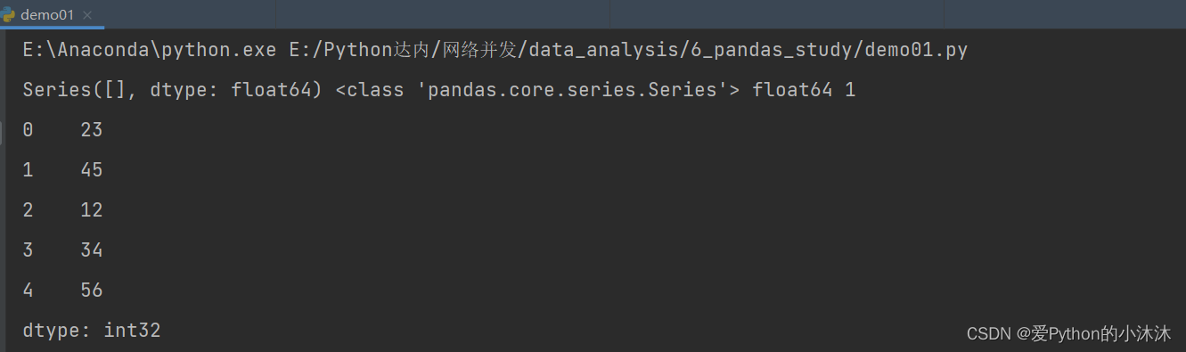
# 1、Series对象创建--空Series对象
s1 = pd.Series()
print(s1, type(s1), s1.dtype, s1.ndim)
# 2、通过ndarray创建Series对象【或者是一个容器,字典时:key值为索引】
ary1 = np.array([23, 45, 12, 34, 56])
s2 = pd.Series(ary1)
print(s2)
输出结果:
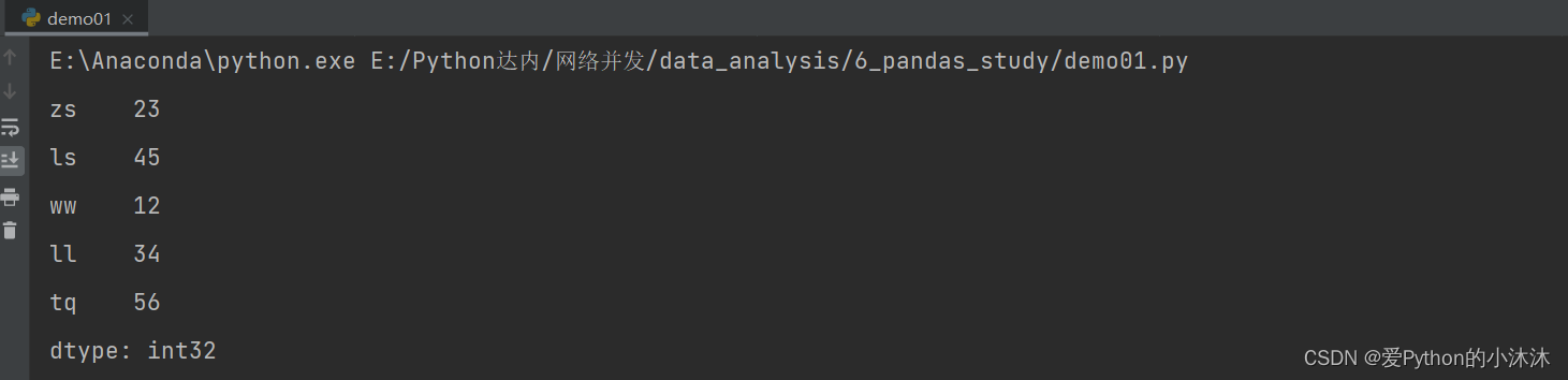
# 3、创建Series对象时,指定index行级索引标签
ary1 = np.array([23, 45, 12, 34, 56])
s3 = pd.Series(ary1, index=['zs', 'ls', 'ww', 'll', 'tq'])
print(s3)
输出结果:
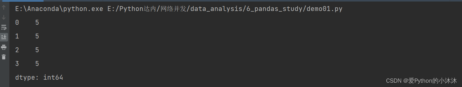
# 5、从标量创建一个系列
s5 = pd.Series(5, index=[0, 1, 2, 3])
print(s5)
输出结果:
1.1.2 Series对象元素的引用
import numpy as np
import pandas as pd
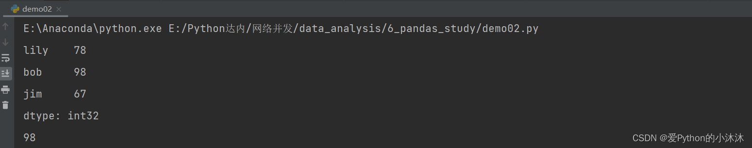
s1 = pd.Series(np.array([78, 98, 67, 100, 76]), index=['lily', 'bob', 'jim', 'jack', 'mary'])
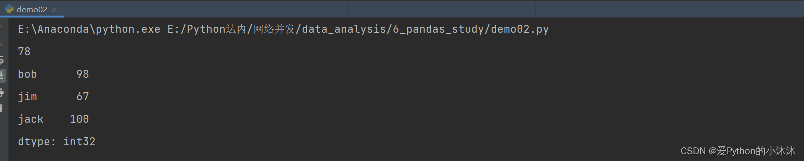
# 方式1:使用索引检索元素
print(s1[:3])  # 返回一个Series对象
print(s1[1])   # 返回value值
输出结果:
# 2、使用标签检索数据[可同时多个元素]
print(s1['lily'])   # 返回value值
print(s1[['bob', 'jim', 'jack']])  # 返回一个Series对象
输出结果:
1.2 日期类型
datetime64[ns] :日期类型
timedelta64[ns] :时间偏移量类型
1.2.1 日期处理
panda识别的日期字符串格式
import pandas as pd
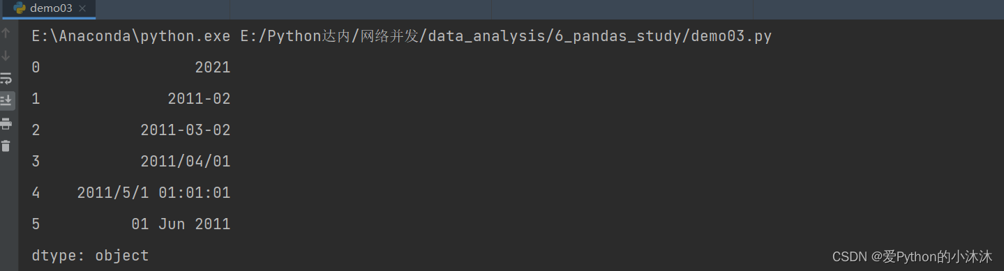
# 将日期列表转为Series对象序列
dates = pd.Series(['2021', '2011-02', '2011-03-02', '2011/04/01', '2011/5/1 01:01:01', '01 Jun 2011'])
print(dates)
输出结果:
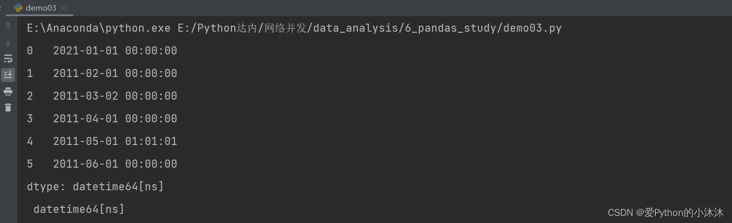
# to_datetime() 转换日期数据类型
dates = pd.to_datetime(dates)
print(dates, '\n', dates.dtype)
输出结果:
datetime类型数据支持日期运算
delta = dates - pd.to_datetime('1970-01-01')
print(delta, type(delta))
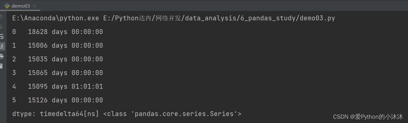
注意–注意:此时Series中的元素类型为timedelta类型
1.2.2 日期相关的操作
测试Series.dt日期相关的操作:具体详细的API参考 help(DatetimeProperties)
import pandas as pd
from pandas.core.indexes.accessors import DatetimeProperties

dates = pd.Series(['2021', '2011-02', '2011-03-02', '2011/04/01', '2011/5/1 01:01:01', '01 Jun 2011'])
dates = pd.to_datetime(dates)
print(dates)
print("*" * 45)
# 获取当前时间的-日
print(dates.dt.day)
print("*" * 45)
# 返回当前日期是每周第几天
print(dates.dt.dayofweek)
print("*" * 45)
# 返回当前日期的秒
print(dates.dt.second)
print(dates.dt.month)
# 返回当前日期是一年的第几周
print(dates.dt.weekofyear)
除上述外,Series.dt还提供了很多日期相关操作
Series.dt.year	The year of the datetime.
Series.dt.month	The month as January=1, December=12.
Series.dt.day	The days of the datetime.
Series.dt.hour	The hours of the datetime.
Series.dt.minute	The minutes of the datetime.
Series.dt.second	The seconds of the datetime.
Series.dt.microsecond	The microseconds of the datetime.
Series.dt.week	The week ordinal of the year.
Series.dt.weekofyear	The week ordinal of the year.
Series.dt.dayofweek	The day of the week with Monday=0, Sunday=6.
Series.dt.weekday	The day of the week with Monday=0, Sunday=6.
Series.dt.dayofyear	The ordinal day of the year.
Series.dt.quarter	The quarter of the date.
Series.dt.is_month_start	Indicates whether the date is the first day of the month.
Series.dt.is_month_end	Indicates whether the date is the last day of the month.
Series.dt.is_quarter_start	Indicator for whether the date is the first day of a quarter.
Series.dt.is_quarter_end	Indicator for whether the date is the last day of a quarter.
Series.dt.is_year_start	Indicate whether the date is the first day of a year.
Series.dt.is_year_end	Indicate whether the date is the last day of the year.
Series.dt.is_leap_year	Boolean indicator if the date belongs to a leap year.
Series.dt.days_in_month	The number of days in the month.
1.3 DateTimeIndex
DateTimeIndex:通过指定周期和频率,使用date_range()函数创建日期序列。默认情况下,范围的频率是天
1.3.1 date_range参数详解
# date_range参数详解
def date_range(
    start=None,       # 生成日期的起始日期
    end=None,         # 结束日期
    periods=None,     # 生成日期序列中日期元素个数
    freq=None,        # 指定生成日期之间的间隔或频率
    tz=None,          # 时区
    normalize=False,
    name=None,
    closed=None,
    **kwargs,
) -> DatetimeIndex
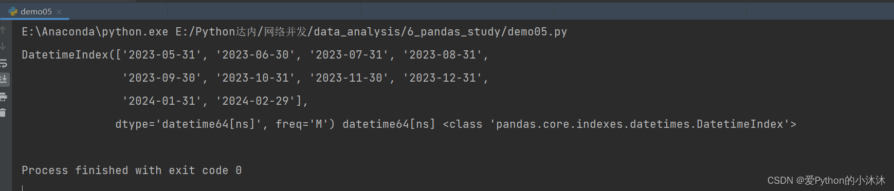
1.3.2 DateTimeIndex创建
# freq="M"代表每月生成一次日期,此种情况首日期从起始日期当月最后一天开始
dates = pd.date_range('2023-5-17', periods=10, freq="M")
print(dates, dates.dtype, type(dates))
输出结果:
1.4 DataFrame
类似于表格的数据类型,可以理解为一个二维数组,索引有两个维度,可更改。
特点:潜在的列是不同的类型;大小可变;标记轴;可以对行和列执行算术运算
1.4.1 DataFrame对象的创建
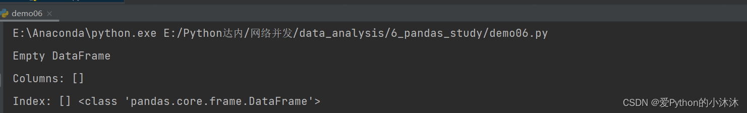
(1)创建一个空对象
# DataFrame对象创建1
df1 = pd.DataFrame()
print(df1, type(df1))
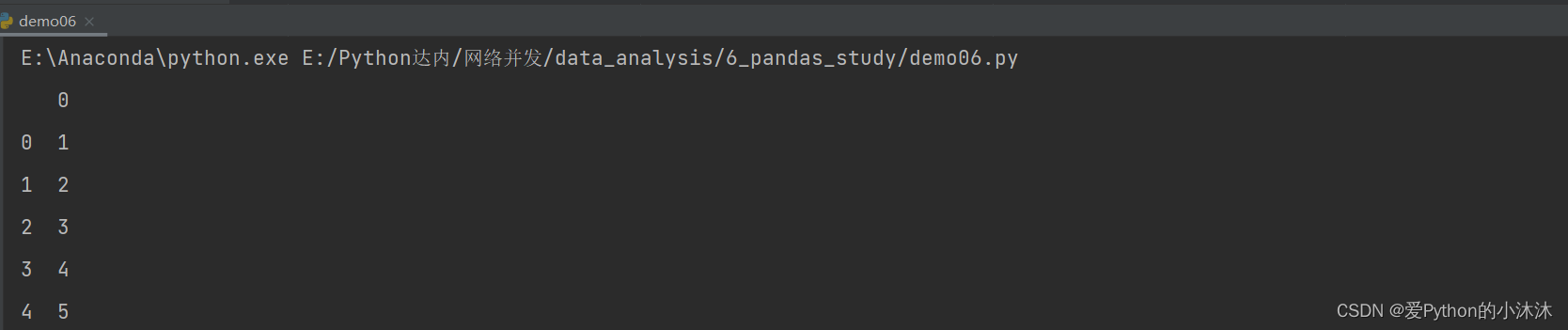
(2)利用一维数组创建DataFrame对象
# DataFrame对象创建[通过一维数组]2
data = [1, 2, 3, 4, 5]
df2 = pd.DataFrame(data)
print(df2)
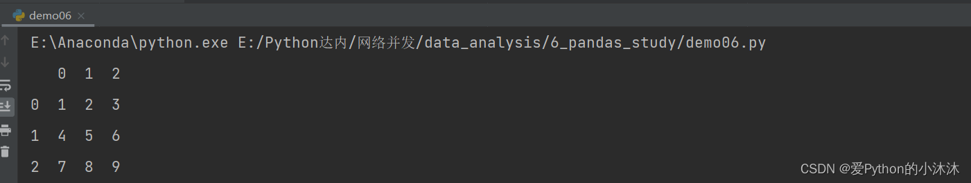
(3)利用二维数组创建DataFrame对象
# DataFrame对象创建[通过二维数组]3
data1 = np.array([1, 2, 3, 4, 5, 6, 7, 8, 9]).reshape(3, 3)
df3 = pd.DataFrame(data1)
print(df3)
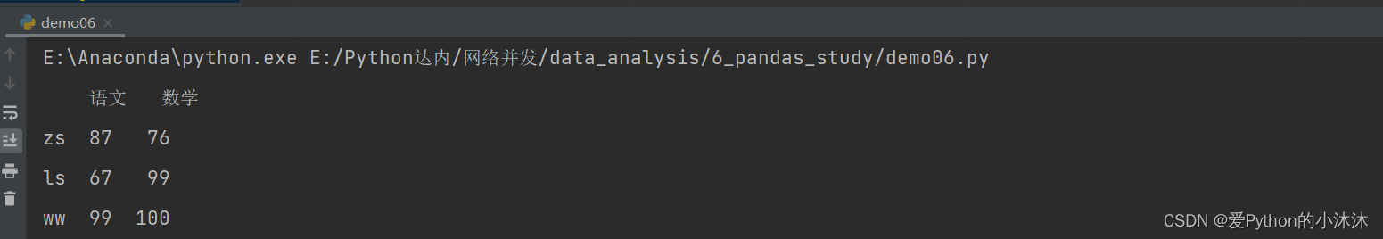
(4)设置行【index】、列索引标签【columns】
# 设置行、列索引标签
data2 = np.array([[87, 76], [67, 99], [99, 100]])
df4 = pd.DataFrame(data2, index=['zs', 'ls', 'ww'], columns=['语文', '数学'])
print(df4)
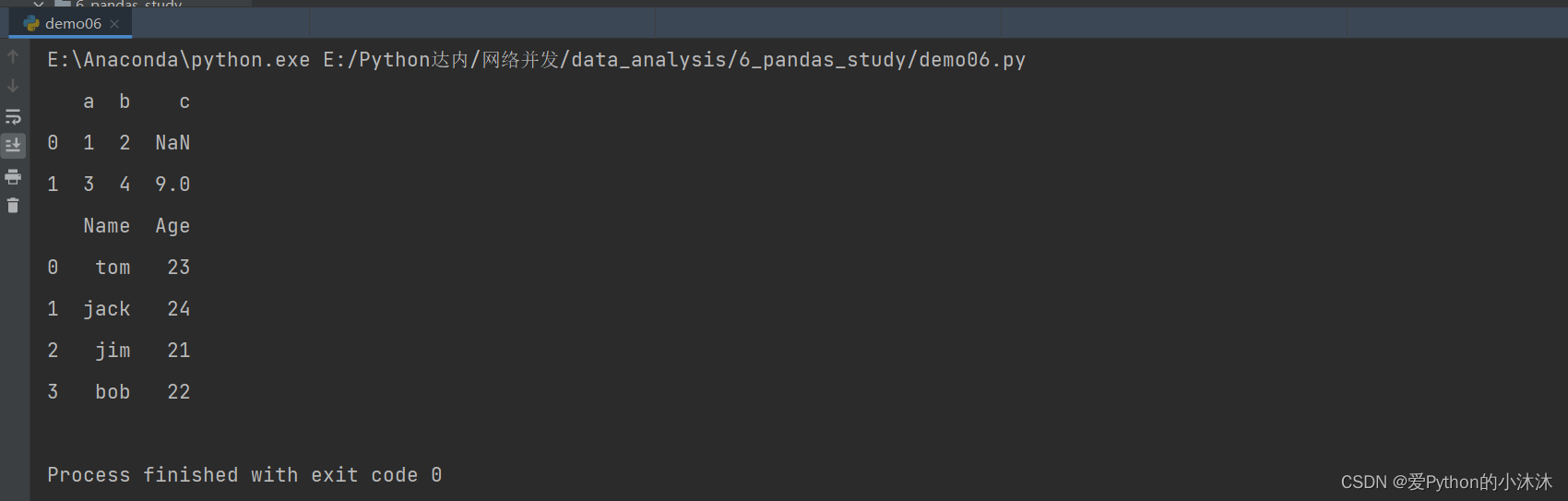
(5)通过字典创建DataFrame对象
# 通过字典创建DataFrame对象
data3 = [{

    'a': 1, 'b': 2}, {

    'a': 3, 'b': 4, 'c': 9}]
print(pd.DataFrame(data3))
data4 = {

    'Name': ['tom', 'jack', 'jim', 'bob'], 'Age': [23, 24, 21, 22]}
print(pd.DataFrame(data4))
(6)可以通过索引标签\索引直接拿到某一行或某一列数据
data4 = {

    'Name': ['tom', 'jack', 'jim', 'bob'], 'Age': [23, 24, 21, 22]}
df5 = pd.DataFrame(data4)
print(df5['Name'])     # 通过列标签拿到'Name'列
2、核心数据结构操作
2.1 列操作
2.1.1 列访问
import numpy as np
import pandas as pd
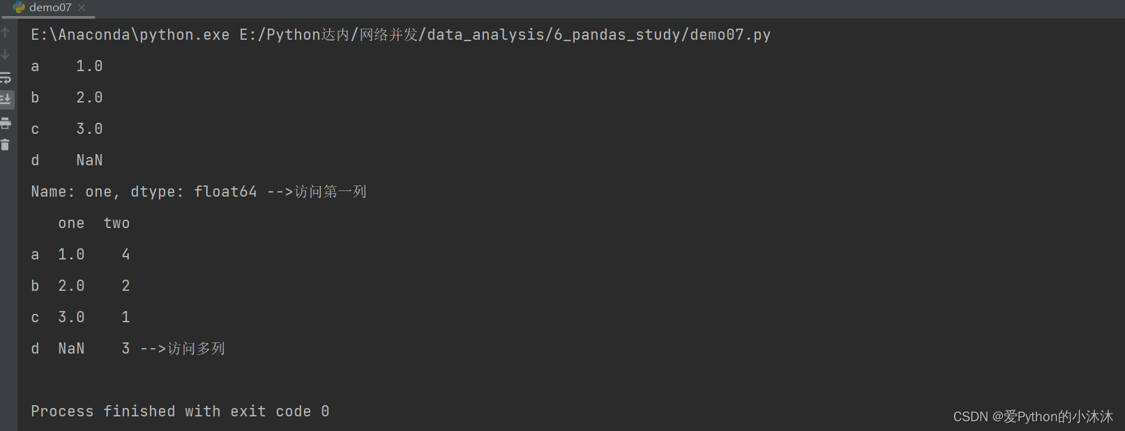
df = pd.DataFrame({
'one': pd.Series([1, 2, 3], index=['a', 'b', 'c']),
'two': pd.Series([1, 2, 3, 4], index={
'a', 'b', 'c', 'd'})})
# 列访问
print(df['one'], '-->访问第一列')
print(df[['one', 'two']], '-->访问多列')
输出结果:
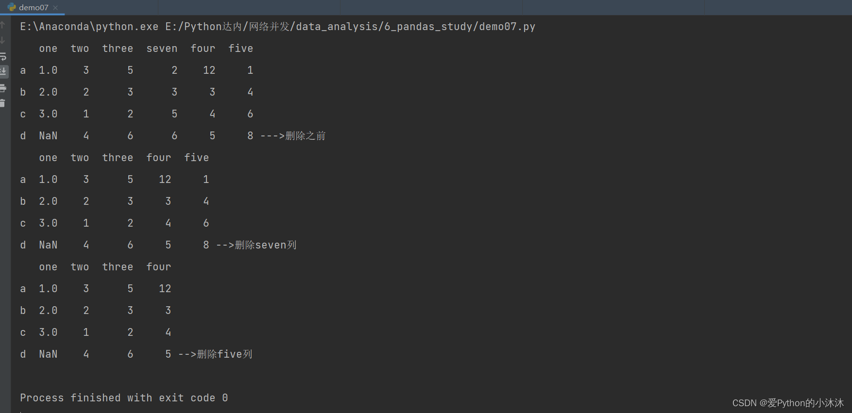
2.1.2 列添加
"""
import numpy as np
import pandas as pd

df = pd.DataFrame({

    'one': pd.Series([1, 2, 3], index=['a', 'b', 'c']),
                   'two': pd.Series([1, 2, 3, 4], index={

    'a', 'b', 'c', 'd'})})
# 列添加
df['three'] = pd.Series([2, 3, 5, 6], index={

    'a', 'b', 'c', 'd'})
# df['six'] = pd.Series([2, 3, 5, 6])  # 使用Series对象添加列时,必须指定索引index,否则默认的0,1,2,3不匹配abcd,都是Nan
df['seven'] = pd.Series([2, 3, 5, 6], index=df.index)
df['four'] = [12, 3, 4, 5]
df['five'] = np.array([1, 4, 6, 8])
print(df)
输出结果:
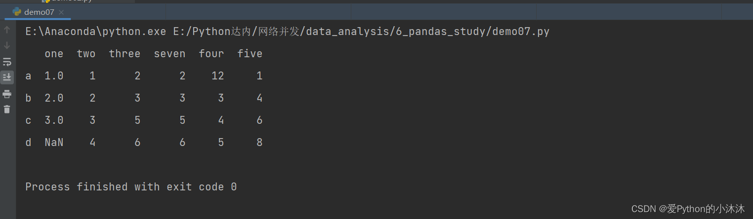
注意:使用Series对象添加列时,必须指定索引index,否则默认的0,1,2,3不匹配abcd,都是Nan
2.1.3 列删除
删除方法常见两种:
方法一:使用pandas中DataFrame类提供的pop方法
方法二:使用del索引的方式删除
df.pop('seven')
print(df, '-->删除seven列')
del (df['five'])
print(df, '-->删除five列')
输出结果:
2.2 行操作
2.2.1 行访问
(1)访问方式1:使用切片
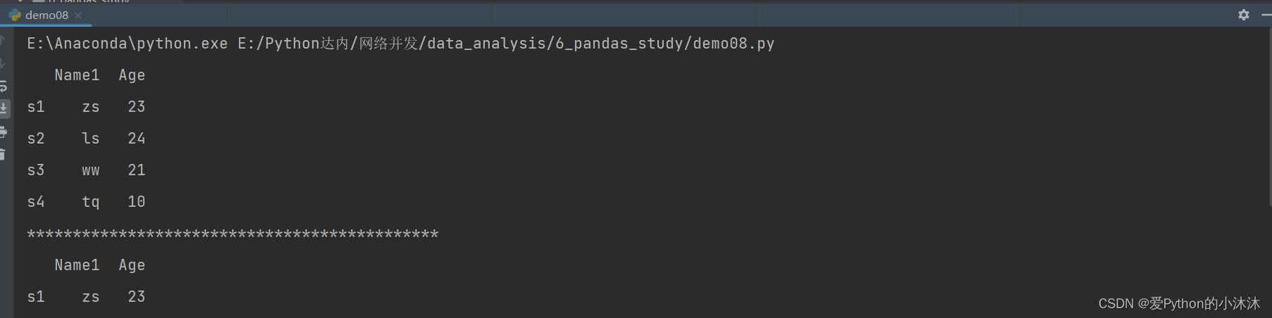
import pandas as pd

name = pd.Series(['zs', 'ls', 'ww', 'tq'], index=['s1', 's2', 's3', 's4'])
age = pd.Series([23, 24, 21, 10], index=['s1', 's2', 's3', 's4'])
df = pd.DataFrame({

    'Name1': name, 'Age': age})
print(df)
print('*' * 45)
# 行访问 使用切片的方式访问
print(df[0:1])   # 访问0行
输出结果:
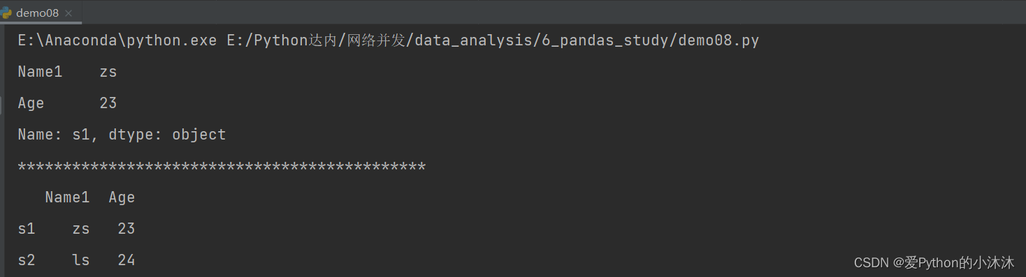
(2)访问方式二:loc方法:针对DataFrame索引名称的切片方法
import pandas as pd

name = pd.Series(['zs', 'ls', 'ww', 'tq'], index=['s1', 's2', 's3', 's4'])
age = pd.Series([23, 24, 21, 10], index=['s1', 's2', 's3', 's4'])
df = pd.DataFrame({

    'Name1': name, 'Age': age})

print(df.loc['s1'])
print('*' * 45)
print(df.loc[['s1', 's2']])
输出结果:
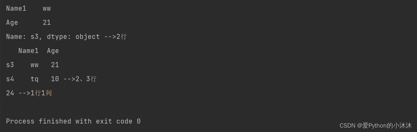
(3)访问方式三:iloc方法,iloc和loc的区别是iloc接受的必须是行索引和列索引的位置。
import pandas as pd

name = pd.Series(['zs', 'ls', 'ww', 'tq'], index=['s1', 's2', 's3', 's4'])
age = pd.Series([23, 24, 21, 10], index=['s1', 's2', 's3', 's4'])
df = pd.DataFrame({

    'Name1': name, 'Age': age})
print(df.iloc[2], '-->2行')
print(df.iloc[[2, 3]], '-->2、3行')  # 2、3行
print(df.iloc[1, 1], '-->1行1列')  # 1行1列
输出结果:
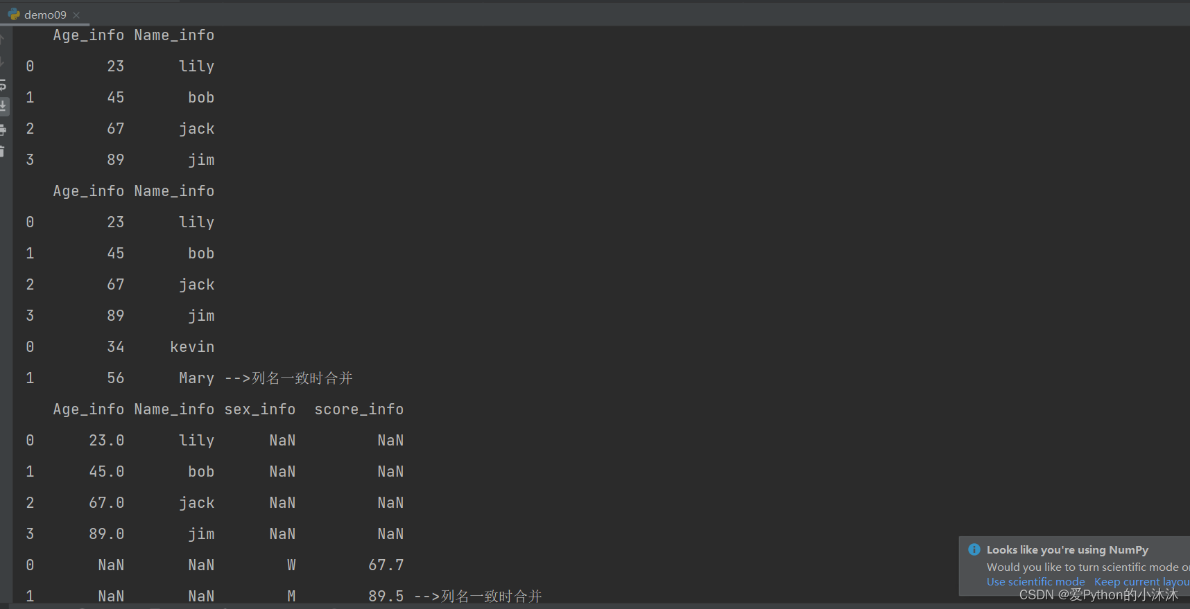
2.2.2 行添加
import numpy as np
import pandas as pd

age = np.array([23, 45, 67, 89])
name = np.array(['lily', 'bob', 'jack', 'jim'])
df = pd.DataFrame({

    'Age_info': age, 'Name_info': name})
print(df)
# df1与df两个DataFrame对象列名一致时,合并操作
df1 = pd.DataFrame({

    'Age_info': pd.Series([34, 56]), 'Name_info': pd.Series(['kevin', 'Mary'])})
# print(df1)
print(df.append(df1))
# df1与df两个DataFrame对象列名不一致时,合并操作
df2 = pd.DataFrame({

    'sex_info': pd.Series(['W', 'M']), 'score_info': pd.Series([67.7, 89.5])})
# print(df2)
print(df.append(df2))
输出结果:
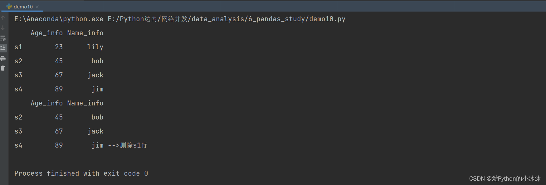
2.2.3 行删除
删除方式:使用索引标签[或无标签使用索引]从DataFrame中删除行。如果标签重复,则会删除多行
注意:使用drop删除后会重新生成一个对象,原对象不变
import numpy as np
import pandas as pd

age = np.array([23, 45, 67, 89])
name = np.array(['lily', 'bob', 'jack', 'jim'])
df = pd.DataFrame({

    'Age_info': age, 'Name_info': name}, index=['s1', 's2', 's3', 's4'])
print(df)
# 使用索引标签[或无标签使用索引]从DataFrame中删除行。如果标签重复,则会删除多行
df1 = df.drop('s1')
print(df1,'-->删除s1行')
输出结果:
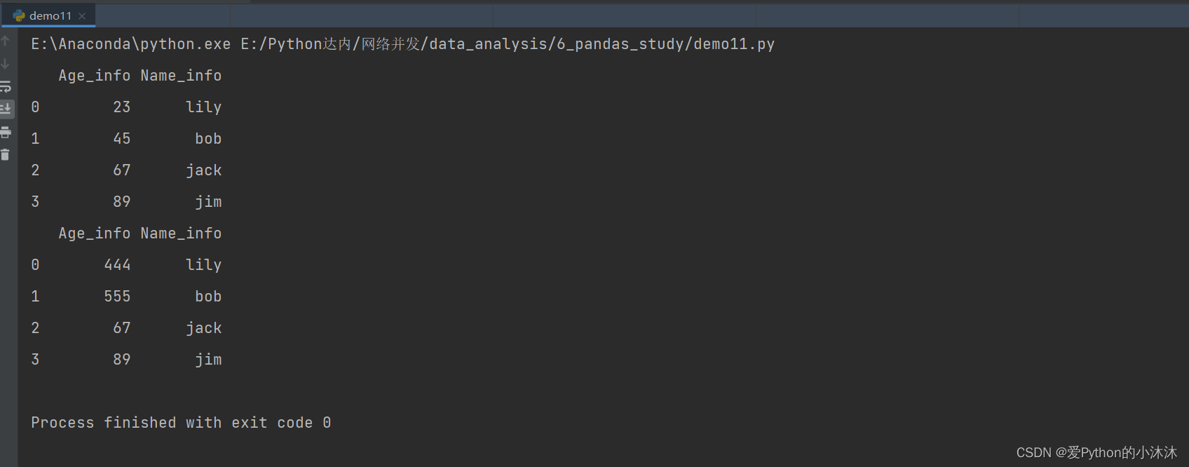
2.3 值修改
(1)方式一:使用loc找到要修改元素
import numpy as np
import pandas as pd

age = np.array([23, 45, 67, 89])
name = np.array(['lily', 'bob', 'jack', 'jim'])
df = pd.DataFrame({

    'Age_info': age, 'Name_info': name})
print(df)
df.loc[0, 'Age_info'] = 444
df.iloc[1, 0] = 555     # 必须是索引,不可以是索引标签
print(df)
输出结果:
(2)SettingWithCopyWarning: A value is trying to be set on a copy of a slice from a DataFrame原因及解决方案
【1】原因:试图改变DataFrame(类似于一个pandas向量)中的一个副本中的值
【2】解决方案:使用loc保证返回的就是其本身,不会产生副本
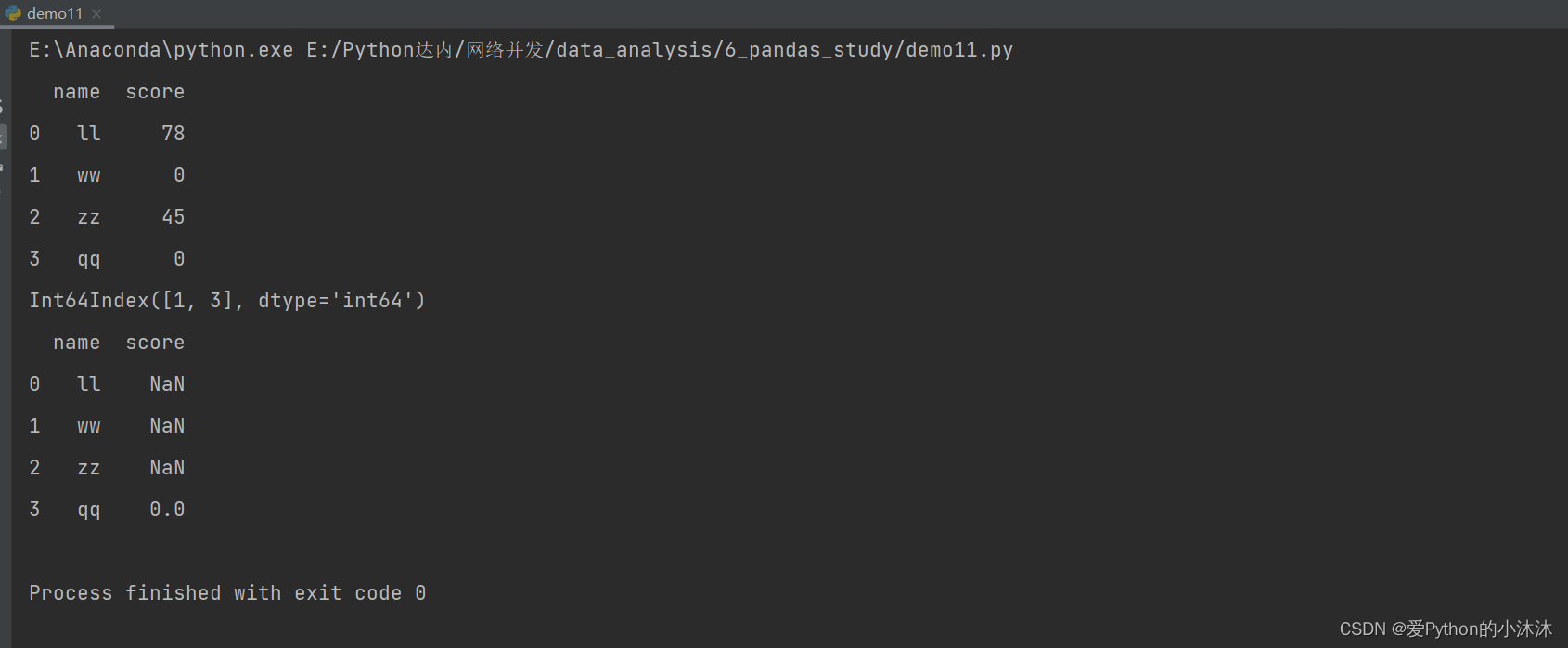
2.4 案例
在DataFrame中掩码依旧可用
案例:将score列中的0值全部修改为np.nan
import numpy as np
import pandas as pd

s1 = pd.Series(['ll', 'ww', 'zz', 'qq'])
s2 = pd.Series([78, 0, 45, 0])
df = pd.DataFrame({

    'name': s1, 'score': s2})
print(df)
mask = df[df['score'] == 0].index   # 查找score为0的行索引,利用了掩码
print(mask)
df.loc[mask, 'score'] = np.nan
print(df)
输出结果:
2.5 DataFrame常用属性
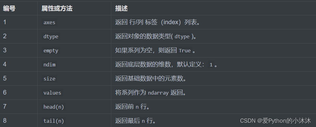
实例代码:
import pandas as pd

data = {

    'Name':['Tom', 'Jack', 'Steve', 'Ricky'],'Age':[28,34,29,42]}
df = pd.DataFrame(data, index=['s1','s2','s3','s4'])
df['score']=pd.Series([90, 80, 70, 60], index=['s1','s2','s3','s4'])
print(df)
print(df.axes)
print(df['Age'].dtype)
print(df.empty)
print(df.ndim)
print(df.size)
print(df.values)
print(df.head(3)) # df的前三行
print(df.tail(3)) # df的后三行
结果演示:
E:\Anaconda\python.exe E:/Python达内/网络并发/data_analysis/6_pandas_study/demo12.py
     Name  Age  score
s1    Tom   28     90
s2   Jack   34     80
s3  Steve   29     70
s4  Ricky   42     60
[Index(['s1', 's2', 's3', 's4'], dtype='object'), Index(['Name', 'Age', 'score'], dtype='object')]
int64
False
2
12
[['Tom' 28 90]
 ['Jack' 34 80]
 ['Steve' 29 70]
 ['Ricky' 42 60]]
     Name  Age  score
s1    Tom   28     90
s2   Jack   34     80
s3  Steve   29     70
     Name  Age  score
s2   Jack   34     80
s3  Steve   29     70
s4  Ricky   42     60

Process finished with exit code 0
3、描述性统计
数值型数据的描述性统计主要包括了计算型数据的完整情况,最小值、最大值、中位数、均值、四分位数、极差、标准差、方差、协方差等。在Numpy库中一些常用的统计学函数也可用于对于数据框架进行描述性统计
3.1 常见API
实例代码:
import pandas as pd

# Create a Dictionary of series
d = {

    'Name': pd.Series(['Tom', 'James', 'Ricky', 'Vin', 'Steve', 'Minsu', 'Jack',
                        'Lee', 'David', 'Gasper', 'Betina', 'Andres', 'Andres']),
     'Age': pd.Series([25, 26, 25, 23, 30, 29, 23, 34, 40, 30, 51, 46, 46]),
     'Rating': pd.Series([4.23, 3.24, 3.98, 2.56, 3.20, 4.6, 3.8, 3.78, 2.98, 4.80, 4.10, 3.65, 3.65]),
     'Score': pd.Series([3.20, 4.6, 3.8, 3.78, 2.98, 4.80, 4.80, 3.65, 4.23, 3.24, 3.98, 2.56, 2.56])}
s = pd.DataFrame({

    'a': pd.Series([4.23, 3.24, 3.98, 2.56, 3.20, 4.6, 3.8, 3.78, 25, 26, 25, 23]),
                  'b': pd.Series([3.20, 4.6, 3.8, 3.78, 2.98, 4.80, 3.8, 3.78, 2.98, 4.80, 4.10, 3.65])})
# Create a DataFrame
df = pd.DataFrame(d)
print(df)
print(df.mean(0))  # 计算平均值 axis代表轴向
print(df.max())
print(df.prod())
print(df.median())  # 中位数
print(df.count())  # 计数
print(df.value_counts())  # 统计每个值出现的次数  查看的是每一行数据出现几次
# print(df.cumprod(), "累积")  # 使用前手动消除非数值型
print(df.std(), '------------------------------标准差')  # 标准差
print(df.cov(), '----协方差')  # 协方差 自动忽略非数值型
print(df.var(), '--------方差')
print(df.corr(), '-------corr')  # 相关系数  任意两对之间的相关系数
print(df.corrwith(s['a']), ' - -----------------corrwith')  # 相关系数 计算每一列与指定对象之间的相关系数,返回Series对象
# print(df.describe())
# print(df.describe(include=['object']))
# print(df.describe(include=['number']))
运行结果:
E:\Anaconda\python.exe E:/Python达内/网络并发/data_analysis/6_pandas_study/demo13.py
      Name  Age  Rating  Score
0      Tom   25    4.23   3.20
1    James   26    3.24   4.60
2    Ricky   25    3.98   3.80
3      Vin   23    2.56   3.78
4    Steve   30    3.20   2.98
5    Minsu   29    4.60   4.80
6     Jack   23    3.80   4.80
7      Lee   34    3.78   3.65
8    David   40    2.98   4.23
9   Gasper   30    4.80   3.24
10  Betina   51    4.10   3.98
11  Andres   46    3.65   2.56
12  Andres   46    3.65   2.56
Age       32.923077
Rating     3.736154
Score      3.706154
dtype: float64
Name      Vin
Age        51
Rating    4.8
Score     4.8
dtype: object
Age      -3.964810e+18
Rating    2.306847e+07
Score     1.894188e+07
dtype: float64
Age       30.00
Rating     3.78
Score      3.78
dtype: float64
Name      13
Age       13
Rating    13
Score     13
dtype: int64
Name    Age  Rating  Score
Andres  46   3.65    2.56     2
Betina  51   4.10    3.98     1
David   40   2.98    4.23     1
Gasper  30   4.80    3.24     1
Jack    23   3.80    4.80     1
James   26   3.24    4.60     1
Lee     34   3.78    3.65     1
Minsu   29   4.60    4.80     1
Ricky   25   3.98    3.80     1
Steve   30   3.20    2.98     1
Tom     25   4.23    3.20     1
Vin     23   2.56    3.78     1
dtype: int64
Age       9.673517
Rating    0.633989
Score     0.773892
dtype: float64 ------------------------------标准差
              Age    Rating     Score
Age     93.576923  0.226346 -3.057821
Rating   0.226346  0.401942  0.004109
Score   -3.057821  0.004109  0.598909 ----协方差
Age       93.576923
Rating     0.401942
Score      0.598909
dtype: float64 --------方差
             Age    Rating     Score
Age     1.000000  0.036907 -0.408458
Rating  0.036907  1.000000  0.008375
Score  -0.408458  0.008375  1.000000 -------corr
Age       0.775174
Rating    0.211911
Score    -0.275430
dtype: float64  - -----------------corrwith

Process finished with exit code 0
3.2 数据去重
(1)DataFrame使用drop_duplicates函数进行去重,参数详解如下:
【1】参数1:subset,默认情况下,对所有列数据同时重复进行识别;或通过subset=[]指定列进行重复识别
【2】参数2:keep,三个可选值{‘first’, ‘last’, False},默认first,表示在识别的重复项中保留按照索引顺序第一项,其余删除;False删除所有重复项
【3】参数3:inplace,False时不对原对象修改,会赋值给新的对象;True对原对象数据进行修改
代码示例:
import pandas as pd

# 通过字典创建DataFrame对象
data = [{

    'name': 'lily', 'age': 24, 'sex': 'M', 'score': 89.7},
        {

    'name': 'jack', 'age': 22, 'sex': 'M', 'score': 76.6},
        {

    'name': 'mary', 'age': 24, 'sex': 'W', 'score': 69.7},
        {

    'name': 'bob', 'age': 22, 'sex': 'M', 'score': 99.7},
        {

    'name': 'james', 'age': 25, 'sex': 'W', 'score': 91},
        {

    'name': 'lily', 'age': 24, 'sex': 'M', 'score': 89.7}]
df = pd.DataFrame(data)
print(df)
# 去除重复数据
# 默认情况下,对于所有的列进行去重,识别重复中保留按照索引顺序的第一个内容,其余删除,不对原数据进行去重,处理结果赋予一个新的变量
df1 = df.drop_duplicates()  # 不修改原数据
print(df1)

df.drop_duplicates(subset=['age', 'sex'], inplace=True)  # 对原对象进行修改,在'age''sex'列识别重复
print(df)
输出结果:
E:\Anaconda\python.exe E:/Python达内/网络并发/data_analysis/6_pandas_study/demo14.py
    name  age sex  score
0   lily   24   M   89.7
1   jack   22   M   76.6
2   mary   24   W   69.7
3    bob   22   M   99.7
4  james   25   W   91.0
5   lily   24   M   89.7
    name  age sex  score
0   lily   24   M   89.7
1   jack   22   M   76.6
2   mary   24   W   69.7
3    bob   22   M   99.7
4  james   25   W   91.0
    name  age sex  score
0   lily   24   M   89.7
1   jack   22   M   76.6
2   mary   24   W   69.7
4  james   25   W   91.0

Process finished with exit code 0
3.3 排序
pandas有两种排序方式,它们分别是按标签和实际值排序
3.3.1 按标签进行排序
用sort_index()方法,传递axis参数和排序顺序,可以对DataFrame进行行排序。默认情况,对行标签进行升序
(1)sort_index()重要参数详解
axis参数:默认值为0,表示按行标签(纵向)排序;1时代表按列标签(水平)排序
ascending参数:默认值True,升序;False时为降序
inplace参数:是否修改原对象,默认False,此时需要新的变量接收此对象;True时,在原对象中修改
(2)代码示例
import numpy as np
import pandas as pd

# np.random.randn(10, 2)生成一个10行2列二维数组
df = pd.DataFrame(np.random.randn(10, 2), index=[8, 2, 4, 6, 1, 7, 0, 5, 3, 9], columns=['col1', 'col2'])
print(df)
# 参数inplace默认False。不在原对象修改;True代表修改原对象
df.sort_index(inplace=True, ascending=False)  # ascending=False时降序
print(df)
输出结果:
E:\Anaconda\python.exe E:/Python达内/网络并发/data_analysis/6_pandas_study/demo15.py
       col1      col2
8 -0.670793 -0.037655
2  0.994857 -2.152398
4  1.304834 -0.292244
6  1.360664  1.097519
1 -0.336153 -0.289120
7 -1.964574  1.090914
0 -1.339923 -1.153182
5 -0.552900  0.279713
3  0.015910 -0.582301
9 -1.666869  0.146527
       col1      col2
9 -1.666869  0.146527
8 -0.670793 -0.037655
7 -1.964574  1.090914
6  1.360664  1.097519
5 -0.552900  0.279713
4  1.304834 -0.292244
3  0.015910 -0.582301
2  0.994857 -2.152398
1 -0.336153 -0.289120
0 -1.339923 -1.153182

Process finished with exit code 0
3.3.2 按实际值排序
用sort_values()方法,参考多列排序时,可以分别指定排序方式
代码示例:
import pandas as pd

# Create a Dictionary of series
d = {

    'Name': pd.Series(['Tom', 'James', 'Ricky', 'Vin', 'Steve', 'Minsu', 'Jack',
                        'Lee', 'David', 'Gasper', 'Betina', 'Andres', 'Andres']),
     'Age': pd.Series([25, 26, 25, 23, 30, 29, 23, 34, 40, 30, 51, 46, 46]),
     'Rating': pd.Series([4.23, 3.24, 3.98, 2.56, 3.20, 4.6, 3.8, 3.78, 2.98, 4.80, 4.10, 3.65, 3.65]),
     'Score': pd.Series([3.20, 4.6, 3.8, 3.78, 2.98, 4.80, 4.80, 3.65, 4.23, 3.24, 3.98, 2.56, 2.56])}
df = pd.DataFrame(d)

print(df)
# 先按Age排序,相同值按Rating排序.Age升序,Rating降序
df.sort_values(by=['Age', 'Rating'], ascending=[True, False], inplace=True)
print(df)
输出结果:
**E:\Anaconda\python.exe E:/Python达内/网络并发/data_analysis/6_pandas_study/demo15.py
      Name  Age  Rating  Score
0      Tom   25    4.23   3.20
1    James   26    3.24   4.60
2    Ricky   25    3.98   3.80
3      Vin   23    2.56   3.78
4    Steve   30    3.20   2.98
5    Minsu   29    4.60   4.80
6     Jack   23    3.80   4.80
7      Lee   34    3.78   3.65
8    David   40    2.98   4.23
9   Gasper   30    4.80   3.24
10  Betina   51    4.10   3.98
11  Andres   46    3.65   2.56
12  Andres   46    3.65   2.56
      Name  Age  Rating  Score
6     Jack   23    3.80   4.80
3      Vin   23    2.56   3.78
0      Tom   25    4.23   3.20
2    Ricky   25    3.98   3.80
1    James   26    3.24   4.60
5    Minsu   29    4.60   4.80
9   Gasper   30    4.80   3.24
4    Steve   30    3.20   2.98
7      Lee   34    3.78   3.65
8    David   40    2.98   4.23
11  Andres   46    3.65   2.56
12  Andres   46    3.65   2.56
10  Betina   51    4.10   3.98

Process finished with exit code 0
**