经典神经网络(1)LeNet及其在Fashion-MNIST数据集上的应用

经典神经网络(1)LeNet

1、卷积神经网络LeNet

之前对于Fashion-MNIST服装分类数据集，为了能够应⽤softmax回归和多层感知机，我们⾸先将每个大小为28 × 28的图像展平为⼀个784维的固定⻓度的⼀维向量，然后⽤全连接层对其进⾏处理，此时我们丢失了图像的空间结构。

pytorch基础操作(四)softmax回归手动实现以及pytorch的API实现

pytorch基础操作(五)多层感知机的实现

通过卷积层的处理⽅法，我们可以在图像中保留空间结构。同时，⽤卷积层代替全连接层的另⼀个好处是：模型更简洁、所需的参数更少。

1.1 LeNet简述

1.1.1 LeNet概述

LeNet是最早发布的卷积神经⽹络之⼀，因其在计算机视觉任务中的⾼效性能⽽受到⼴泛关注。这个模型是由AT&T⻉尔实验室的研究员Yann LeCun在1989年提出的（并以其命名），⽬的是识别图像中的⼿写数字。

当时，LeNet取得了与⽀持向量机（support vector machines）性能相媲美的成果，成为监督学习的主流⽅法。LeNet被⼴泛⽤于⾃动取款机（ATM）机中，帮助识别处理⽀票的数字。

1.1.2 LeNet的原始的网络架构

注：feature map 的描述有两种：channel first，如256x3x3；channel last，如3x3x256 。

LeNet 网络包含了卷积层、池化层、全连接层，这些都是现代CNN 网络的基本组件。

• 输入层：二维图像，尺寸为32x32。

• C1、C3、C5 层：二维卷积层。

  扫描二维码关注公众号，回复： 15374311 查看本文章

  其中C5 将输入的 feature map（尺寸 16@5x5 ）转化为尺寸为120x1x1 的 feature map，然后转换为长度为120 的一维向量。

  这是一种常见的、将卷积层的输出转换为全连接层的输入的一种方法。

• S2、S4 层：池化层。使用sigmoid 函数作为激活函数。

  后续的 CNN 都使用ReLU 作为激活函数。

• F6 层：全连接层。

• 输出层：由欧式径向基函数单元组成。

  后续的CNN 使用softmax 输出单元。

网络层	核/池大小	核数量	步长	输入尺寸	输出尺寸
INPUT	-	-	-	-	1@32x32
C1	5x5	6	1	1@32x32	6@28x28
S2	2x2	-	2	6@28x28	6@14x14
C3	5x5	16	1	6@14x14	16@10x10
S4	2x2	-	2	16@10x10	16@5x5
C5	5x5	120	1	16@5x5	120@1x1
F6	-	-	-	120	84
OUTPUT	-	-	-	84	10

1.2 架构图解释

我们将对原始模型做了⼀点⼩改动，去掉了最后⼀层的⾼斯激活，简化为下图。

• 每个卷积块中的基本单元是⼀个卷积层、⼀个sigmoid激活函数和平均汇聚层。请注意，虽然ReLU和最⼤汇聚层更有效，但它们在20世纪90年代还没有出现。

• 每个卷积层使⽤5 × 5卷积核和⼀个sigmoid激活函数。这些层将输⼊映射到多个⼆维特征输出，通常同时增加通道的数量。第⼀卷积层有6个输出通道，⽽第⼆个卷积层有16个输出通道。每个2 × 2池操作（步幅2）通过空间下采样将维数减少4倍。卷积的输出形状由批量⼤大小、通道数、高度、宽度决定。

• 为了将卷积块的输出传递给稠密块，我们必须在⼩批量中展平每个样本。我们将这个四维输⼊转换成全连接层所期望的⼆维输⼊。这⾥的⼆维表示的第⼀个维度索引小批量中的样本，第⼆个维度给出每个样本的平⾯向量表⽰。LeNet的稠密块有三个全连接层，分别有120、84和10个输出。因为我们在执⾏分类任务，所以输出层的10维对应于最后输出结果的数量。

1.3 LeNet在Fashion-MNIST数据集上的应用代码

1.3.1 定义LeNet模型

import torch.nn as nn
import torch

class LeNet5(nn.Module):

    def __init__(self):
        super().__init__()
        self.model = nn.Sequential(
            nn.Conv2d(in_channels=1, out_channels=6, kernel_size=5, padding=2, stride=1),
            nn.Sigmoid(),
            nn.AvgPool2d(kernel_size=2,stride=2),
            nn.Conv2d(in_channels=6, out_channels=16, kernel_size=5),
            nn.Sigmoid(),
            nn.AvgPool2d(kernel_size=2,stride=2),
            nn.Flatten(),
            nn.Linear(in_features=16 * 5 * 5, out_features=120),
            nn.Sigmoid(),
            nn.Linear(in_features=120, out_features=84),
            nn.Sigmoid(),
            nn.Linear(in_features=84, out_features=10)
        )

    def forward(self, X):
        X = self.model(X)
        return X



if __name__ == '__main__':
    net = LeNet5()
    # 测试神经网络是否可运行
    # inputs = torch.rand(size=(1, 1, 28, 28), dtype=torch.float32)
    # outputs = net(inputs)
    # print(outputs.shape)
    # 查看每一层输出的shape
    X = torch.rand(size=(1, 1, 28, 28), dtype=torch.float32)
    for layer in net.model:
        X = layer(X)
        print(layer.__class__.__name__, 'output shape:', X.shape)

Conv2d output shape: torch.Size([1, 6, 28, 28])
Sigmoid output shape: torch.Size([1, 6, 28, 28])
AvgPool2d output shape: torch.Size([1, 6, 14, 14])
Conv2d output shape: torch.Size([1, 16, 10, 10])
Sigmoid output shape: torch.Size([1, 16, 10, 10])
AvgPool2d output shape: torch.Size([1, 16, 5, 5])
Flatten output shape: torch.Size([1, 400])
Linear output shape: torch.Size([1, 120])
Sigmoid output shape: torch.Size([1, 120])
Linear output shape: torch.Size([1, 84])
Sigmoid output shape: torch.Size([1, 84])
Linear output shape: torch.Size([1, 10])

• 在整个卷积块中，与上⼀层相⽐，每⼀层特征的⾼度和宽度都减⼩了。

  • 第⼀个卷积层使⽤2个像素的填充，来补偿5 × 5卷积核导致的特征减少。

  • 第⼆个卷积层没有填充，因此⾼度和宽度都减少了4个像素。

• 随着层叠的上升，通道的数量从输⼊时的1个，增加到第⼀个卷积层之后的6个，再到第⼆个卷积层之后的16个。同时，每个汇聚层的⾼度和宽度都减半。

• 最后，每个全连接层减少维数，最终输出⼀个维数与结果分类数相匹配的输出。

1.3.2 读取Fashion-MNIST数据集

# 通过框架中的内置函数将Fashion-MNIST数据集下载并读取到内存中
# Fashion-MNIST是⼀个服装分类数据集，由10个类别的图像组成
# Fashion-MNIST由10个类别的图像组成，每个类别由训练数据集（train dataset）中的6000张图像和测试数据集（test dataset）中的1000张图像组成。
# 因此，训练集和测试集分别包含60000和10000张图像。

'''
  读取服装分类数据集 Fashion-MNIST
'''
import torchvision
import torch
from torch.utils import data
from torchvision import transforms

def get_dataloader_workers():
    """使⽤4个进程来读取数据"""
    return 4

def get_mnist_data(batch_size, resize=None):
    trans = [transforms.ToTensor()]

    if resize:
        # 还接受⼀个可选参数resize，⽤来将图像⼤⼩调整为另⼀种形状
        trans.insert(0,transforms.Resize(resize))
    trans = transforms.Compose(trans)

    # 需要下载，可以设置为True
    mnist_train = torchvision.datasets.FashionMNIST(
        root='./data',train=True,transform=trans,download=False
    )


    mnist_test = torchvision.datasets.FashionMNIST(
        root='./data',train=False,transform=trans,download=False
    )
    # 数据加载器每次都会读取⼀⼩批量数据，⼤⼩为batch_size。通过内置数据迭代器，我们可以随机打乱了所有样本，从⽽⽆偏⻅地读取⼩批量
    # 数据迭代器是获得更⾼性能的关键组件。依靠实现良好的数据迭代器，利⽤⾼性能计算来避免减慢训练过程。
    train_iter = data.DataLoader(mnist_train,batch_size=batch_size,shuffle=True,num_workers=get_dataloader_workers())
    test_iter = data.DataLoader(mnist_test,batch_size=batch_size,shuffle=True,num_workers=get_dataloader_workers())

    return (train_iter,test_iter)


batch_size = 256

train_iter,test_iter = get_mnist_data(batch_size)

1.3.3 定义通用的网络模型训练函数

1、先定义几个类，用来计算精确率，画图，计算训练时间等

累加类Accumulator

'''
定义⼀个实⽤程序类Accumulator，⽤于对多个变量进⾏累加
'''
class Accumulator():

    """在n个变量上累加"""
    def __init__(self, n):
        self.data = [0.0] * n


    def add(self, *args):
        self.data = [a + float(b) for a,b in zip(self.data, args)]


    def reset(self):
        self.data = [0.0] * len(self.data)

    def __getitem__(self,index):
        return self.data[index]

时间类Timer

import time

class Timer:
    """Record multiple running times."""
    def __init__(self):
        """Defined in :numref:`subsec_linear_model`"""
        self.times = []
        self.start()

    def start(self):
        """Start the timer."""
        self.tik = time.time()

    def stop(self):
        """Stop the timer and record the time in a list."""
        self.times.append(time.time() - self.tik)
        return self.times[-1]

    def avg(self):
        """Return the average time."""
        return sum(self.times) / len(self.times)

    def sum(self):
        """Return the sum of time."""
        return sum(self.times)

    def cumsum(self):
        """Return the accumulated time."""
        return np.array(self.times).cumsum().tolist()

绘图类Animator

from matplotlib import pyplot as plt
from IPython import display


def set_axes(axes, xlabel, ylabel, xlim, ylim, xscale, yscale, legend):
    """设置matplotlib的轴"""
    axes.set_xlabel(xlabel)
    axes.set_ylabel(ylabel)
    axes.set_xscale(xscale)
    axes.set_yscale(yscale)
    axes.set_xlim(xlim)
    axes.set_ylim(ylim)
    if legend:
        axes.legend(legend)
    axes.grid()

class Animator():
    """在动画中绘制数据"""
    def __init__(self, xlabel=None, ylabel=None, legend=None, xlim=None,
                 ylim=None, xscale='linear', yscale='linear',
                 fmts=('-', 'm--', 'g-.', 'r:'), nrows=1, ncols=1,
                 figsize=(3.5, 2.5)):


        # 增量地绘制多条线
        if legend is None:
            legend = []
        self.fig, self.axes = plt.subplots(nrows, ncols, figsize=figsize)
        if nrows * ncols == 1:
            self.axes = [self.axes, ]
        # 使用lambda函数捕获参数
        self.config_axes = lambda: set_axes(
            self.axes[0], xlabel, ylabel, xlim, ylim, xscale, yscale, legend)
        self.X, self.Y, self.fmts = None, None, fmts

    def add(self, x, y):
        # 向图表中添加多个数据点
        if not hasattr(y, "__len__"):
            y = [y]
        n = len(y)
        if not hasattr(x, "__len__"):
            x = [x] * n
        if not self.X:
            self.X = [[] for _ in range(n)]
        if not self.Y:
            self.Y = [[] for _ in range(n)]
        for i, (a, b) in enumerate(zip(x, y)):
            if a is not None and b is not None:
                self.X[i].append(a)
                self.Y[i].append(b)
        self.axes[0].cla()
        for x, y, fmt in zip(self.X, self.Y, self.fmts):
            self.axes[0].plot(x, y, fmt)
        self.config_axes()
        display.display(self.fig)
        display.clear_output(wait=True)

2、定义训练函数

import torch.nn as nn
from AccumulatorClass import Accumulator

def accuracy(y_hat, y):
    """计算预测正确的数量"""
    if len(y_hat.shape) > 1 and y_hat.shape[1] > 1:
         y_hat = y_hat.argmax(axis=1)
    cmp = y_hat.type(y.dtype) == y
    return float(cmp.type(y.dtype).sum())



def evaluate_accuracy_gpu(net, data_iter, device=None):
    """使⽤GPU计算模型在数据集上的精度"""
    if isinstance(net, nn.Module):
        net.eval() # 设置为评估模式
        if not device:
            device = next(iter(net.parameters())).device
    # 正确预测的数量，总预测的数量
    metric = Accumulator(2)
    with torch.no_grad():
        for X, y in data_iter:
            if isinstance(X, list):
                # BERT微调所需的
                X = [x.to(device) for x in X]
            else:
                X = X.to(device)
            y = y.to(device)
            metric.add(accuracy(net(X), y), y.numel())
    return metric[0] / metric[1]

from AnimatorClass import Animator
from TimerClass import Timer

def train_ch(net, train_iter, test_iter, num_epochs, lr, device):
    """⽤GPU训练模型"""
    def init_weights(m):
        if type(m) == nn.Linear or type(m) == nn.Conv2d:
            nn.init.xavier_uniform_(m.weight)
    # 初始化权重
    net.apply(init_weights)
    print('training on', device)
   
    net.to(device)
    # 梯度下降
    optimizer = torch.optim.SGD(net.parameters(), lr=lr)
    # 交叉熵损失
    loss = nn.CrossEntropyLoss()

    animator = Animator(xlabel='epoch', xlim=[1, num_epochs],legend=['train loss', 'train acc', 'test acc'])
    timer, num_batches = Timer(), len(train_iter)
    num_batches = len(train_iter)
    for epoch in range(num_epochs):
        # 训练损失之和，训练准确率之和，样本数
        metric = Accumulator(3)
        net.train()
        for i, (X, y) in enumerate(train_iter):
            timer.start()
            optimizer.zero_grad()
            X, y = X.to(device), y.to(device)
            y_hat = net(X)
            l = loss(y_hat, y)
            l.backward()
            optimizer.step()
            with torch.no_grad():
                metric.add(l * X.shape[0], accuracy(y_hat, y), X.shape[0])
            timer.stop()
            train_l = metric[0] / metric[2]
            train_acc = metric[1] / metric[2]
            if (i + 1) % (num_batches // 5) == 0 or i == num_batches - 1:
                animator.add(epoch + (i + 1) / num_batches,(train_l, train_acc, None))

        test_acc = evaluate_accuracy_gpu(net, test_iter)
        animator.add(epoch + 1, (None, None, test_acc))
    print(f'loss {
      
      train_l:.3f}, train acc {
      
      train_acc:.3f}, test acc {
      
      test_acc:.3f}')
    print(f'{
      
      metric[2] * num_epochs / timer.sum():.1f} examples/sec on {
      
      str(device)}')

1.3.4 利用LeNet进行训练

from _01_LeNet5 import LeNet5

def try_gpu(i=0):
    if torch.cuda.device_count() >= i + 1:
        return torch.device(f'cuda:{
      
      i}')
    return torch.device('cpu')

# 初始化模型
net = LeNet5()

lr, num_epochs = 0.9, 10
train_ch(net, train_iter, test_iter, num_epochs, lr, try_gpu())

结果如下：

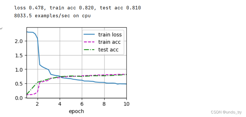
这是唯一的能用自己电脑的cpu跑的动的模型了，以后的AlexNet、Vgg等都跑不动，需要用GPU加速计算。如果自己电脑没有显卡，可以去colab白嫖，也可以租一个GPU，例如AutoDL平台，可以参考下面博客租借

AutoDL平台租借GPU详解

注：卷积神经网络通俗解释

大白话讲解卷积神经网络工作原理

从“卷积”、到“图像卷积操作”、再到“卷积神经网络”，“卷积”意义的3次改变