一般的深度学习入门例子是 MNIST 的训练和测试,几乎就算是深度学习领域的 HELLO WORLD 了,但是,有一个问题是,MNIST 太简单了,初学者闭着眼镜随便构造几层网络就可以将准确率提升到 90% 以上。但是,初学者这算入门了吗?
答案是没有。
现实开发当中的例子可没有这么简单,如果让初学者直接去上手 VOC 或者是 COCO 这样的数据集,很可能自己搭建的神经网络准确率不超过 30%。
是的,如果不用开源的 VGG、GooLeNet、ResNet 等等,也许你手下敲出的代码命中率还没有瞎猜高。
这篇文章介绍如何用 Pytorch 训练一个自建的神经网络去训练 Fashion-MNIST 数据集。
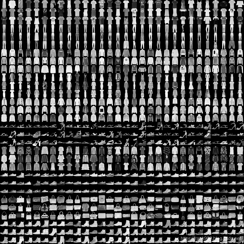
Fashion-MNIST
Fashion-MINST 的目的是为了替代 MNIST。
这是它的地址:https://github.com/zalandoresearch/fashion-mnist
它是一系列的服装图片集合,总共有 10 个类别。
60000 张训练图片,10000 张测试图片。
| Label | Description |
|---|---|
| 0 | T-shirt/top |
| 1 | Trouser |
| 2 | Pullover |
| 3 | Dress |
| 4 | Coat |
| 5 | Sandal |
| 6 | Shirt |
| 7 | Sneaker |
| 8 | Bag |
| 9 | Ankle boo |
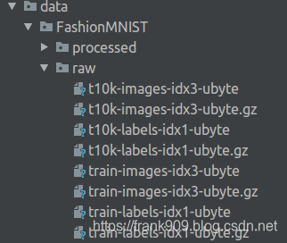
Fashion-MNIST 体积并不大,更方便的是像 Tensorflow 和 Pytorch 目前的版本都可以直接用代码下载。
训练神经网络的步骤
下面我张图是我自己制作的,每次要写相关博客时,我都会翻出来温习一下。
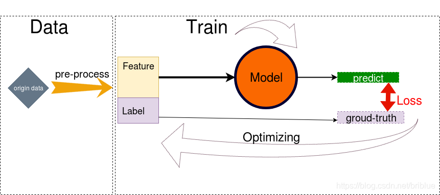
它会提醒我要做这些事情:
- 处理数据
- 搭建模型
- 确定 Loss 函数
- 训练
下面文章就按这样的步骤来讲解
处理数据
下载数据
Pytorch 现在通过现成的 API 就可以下载 Fashion-MINST 的数据
trainset = torchvision.datasets.FashionMNIST(root='./data', train=True,
                                        download=True, transform=transform)
trainloader = torch.utils.data.DataLoader(trainset, batch_size=100,
                                          shuffle=True, num_workers=2)

testset = torchvision.datasets.FashionMNIST(root='./data', train=False,
                                       download=True, transform=transform1)
testloader = torch.utils.data.DataLoader(testset, batch_size=50,
                                         shuffle=False, num_workers=2)
上面创建了两个 DataLoader ,分别用来加载训练集的图片和测试集的图片。
代码运行后,会在当前目录的 data 目录下存放对应的文件。
数据增强
为提高模型的泛化能力,一般会将数据进行增强操作。
transform = transforms.Compose(
    [
     transforms.RandomHorizontalFlip(),
     transforms.RandomGrayscale(),
     transforms.ToTensor()])

transform1 = transforms.Compose(
    [
     transforms.ToTensor()])
transform 主要进行了左右翻转,灰度随机变换,用来给训练的图像进行数据加强,测试的图片就不需要了。
transform 的引用传递到前面的数据集对应的 API 就可以了,非常方便。
搭建模型
虽然是自己搭建的神经网络,但是却参考了 VGG 的网络架构。
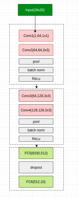
总共 6 层网络,4 层卷积层,2 层全连接。
用 Pytorch 实现起来也非常方便。
class Net(nn.Module):


    def __init__(self):
        super(Net,self).__init__()
        self.conv1 = nn.Conv2d(1,64,1,padding=1)
        self.conv2 = nn.Conv2d(64,64,3,padding=1)
        self.pool1 = nn.MaxPool2d(2, 2)
        self.bn1 = nn.BatchNorm2d(64)
        self.relu1 = nn.ReLU()

        self.conv3 = nn.Conv2d(64,128,3,padding=1)
        self.conv4 = nn.Conv2d(128, 128, 3,padding=1)
        self.pool2 = nn.MaxPool2d(2, 2, padding=1)
        self.bn2 = nn.BatchNorm2d(128)
        self.relu2 = nn.ReLU()

        self.fc5 = nn.Linear(128*8*8,512)
        self.drop1 = nn.Dropout2d()
        self.fc6 = nn.Linear(512,10)


    def forward(self,x):
        x = self.conv1(x)
        x = self.conv2(x)
        x = self.pool1(x)
        x = self.bn1(x)
        x = self.relu1(x)


        x = self.conv3(x)
        x = self.conv4(x)
        x = self.pool2(x)
        x = self.bn2(x)
        x = self.relu2(x)

        #print(" x shape ",x.size())
        x = x.view(-1,128*8*8)
        x = F.relu(self.fc5(x))
        x = self.drop1(x)
        x = self.fc6(x)

        return x
值得注意的是,在卷积层后我使用了 Batch Norm 的手段,在全连接层我使用了 Dropout,两者的目的都是为了降低过拟合的现象。
制定训练策略
我选用了比较流行的 Adam 作为优化有段,学习率 是 0.0001。
然后,loss 选用 交叉熵。
    def train_sgd(self,device,epochs=100):
        optimizer = optim.Adam(self.parameters(), lr=0.0001)

        path = 'weights.tar'
        initepoch = 0

        if os.path.exists(path) is not True:
            loss = nn.CrossEntropyLoss()
            # optimizer = optim.SGD(self.parameters(),lr=0.01)

        else:
            checkpoint = torch.load(path)
            self.load_state_dict(checkpoint['model_state_dict'])
            optimizer.load_state_dict(checkpoint['optimizer_state_dict'])
            initepoch = checkpoint['epoch']
            loss = checkpoint['loss']


        for epoch in range(initepoch,epochs):  # loop over the dataset multiple times
            timestart = time.time()

            running_loss = 0.0
            total = 0
            correct = 0
            for i, data in enumerate(trainloader, 0):
                # get the inputs
                inputs, labels = data
                inputs, labels = inputs.to(device),labels.to(device)

                # zero the parameter gradients
                optimizer.zero_grad()

                # forward + backward + optimize
                outputs = self(inputs)
                l = loss(outputs, labels)
                l.backward()
                optimizer.step()

                # print statistics
                running_loss += l.item()
                # print("i ",i)
                if i % 500 == 499:  # print every 500 mini-batches
                    print('[%d, %5d] loss: %.4f' %
                          (epoch, i, running_loss / 500))
                    running_loss = 0.0
                    _, predicted = torch.max(outputs.data, 1)
                    total += labels.size(0)
                    correct += (predicted == labels).sum().item()
                    print('Accuracy of the network on the %d tran images: %.3f %%' % (total,
                            100.0 * correct / total))
                    total = 0
                    correct = 0
                    torch.save({'epoch':epoch,
                                'model_state_dict':net.state_dict(),
                                'optimizer_state_dict':optimizer.state_dict(),
                                'loss':loss
                                },path)

            print('epoch %d cost %3f sec' %(epoch,time.time()-timestart))

        print('Finished Training')
上面这段代码中也有保存和加载模型的功能。
通过 save()
可以保存网络训练状态。
torch.save({'epoch':epoch,
             'model_state_dict':net.state_dict(),
             'optimizer_state_dict':optimizer.state_dict(),
             'loss':loss
             },path)
我在代码中定义了 path 为 weights.tar,任务执行时,模型数据也会保存下来。
通过load()
可以加载保存的模型数据。
checkpoint = torch.load(path)
            self.load_state_dict(checkpoint['model_state_dict'])
            optimizer.load_state_dict(checkpoint['optimizer_state_dict'])
            initepoch = checkpoint['epoch']
            loss = checkpoint['loss']
测试
测试和训练有些不同,它只需要前向推导就好了。
    def test(self,device):
        correct = 0
        total = 0
        with torch.no_grad():
            for data in testloader:
                images, labels = data
                images, labels = images.to(device), labels.to(device)
                outputs = self(images)
                _, predicted = torch.max(outputs.data, 1)
                total += labels.size(0)
                correct += (predicted == labels).sum().item()

        print('Accuracy of the network on the 10000 test images: %.3f %%' % (
                100.0 * correct / total))
训练结果
下面编写代码进行训练和验证。
if __name__ == "__main__":

    device = torch.device("cuda:0" if torch.cuda.is_available() else "cpu")
    net = Net()
    net = net.to(device)
    net.train_sgd(device,30)
    net.test(device)
代码会根据机器有没有 cuda 设备来决定用什么训练,比如机器没有安装 GPU,那么就会用 CPU 执行,速度会稍慢一点。
因为模型简单,我选择了训练 30 个 epoch 就终止。
最后,就可以运行代码了。
我的 Pytorch 版本是 1.2,Cuda 版本是 10.1,GPU 是 1080 Ti.
跑一个 epoch 的时间大概花费 6 秒多。
经过 30 个 epoch 之后,训练准确度可以达到 99%,测试准确率可以为 92.29%.
[0,   499] loss: 0.4572
Accuracy of the network on the 100 tran images: 87.000 %
epoch 0 cost 7.158301 sec
[1,   499] loss: 0.2840
Accuracy of the network on the 100 tran images: 90.000 %
epoch 1 cost 6.451613 sec
[2,   499] loss: 0.2458
Accuracy of the network on the 100 tran images: 95.000 %
epoch 2 cost 6.450977 sec
[3,   499] loss: 0.2197
Accuracy of the network on the 100 tran images: 92.000 %
epoch 3 cost 6.383819 sec
[4,   499] loss: 0.2009
Accuracy of the network on the 100 tran images: 90.000 %
epoch 4 cost 6.443048 sec
[5,   499] loss: 0.1840
Accuracy of the network on the 100 tran images: 94.000 %
epoch 5 cost 6.411542 sec
[6,   499] loss: 0.1688
Accuracy of the network on the 100 tran images: 94.000 %
epoch 6 cost 6.420368 sec
[7,   499] loss: 0.1584
Accuracy of the network on the 100 tran images: 93.000 %
epoch 7 cost 6.390420 sec
[8,   499] loss: 0.1452
Accuracy of the network on the 100 tran images: 93.000 %
epoch 8 cost 6.473319 sec
[9,   499] loss: 0.1342
Accuracy of the network on the 100 tran images: 96.000 %
epoch 9 cost 6.435586 sec
[10,   499] loss: 0.1275
Accuracy of the network on the 100 tran images: 95.000 %
epoch 10 cost 6.422722 sec
[11,   499] loss: 0.1177
Accuracy of the network on the 100 tran images: 96.000 %
epoch 11 cost 6.490834 sec
[12,   499] loss: 0.1085
Accuracy of the network on the 100 tran images: 96.000 %
epoch 12 cost 6.499629 sec
[13,   499] loss: 0.1021
Accuracy of the network on the 100 tran images: 92.000 %
epoch 13 cost 6.512994 sec
[14,   499] loss: 0.0929
Accuracy of the network on the 100 tran images: 96.000 %
epoch 14 cost 6.510045 sec
[15,   499] loss: 0.0871
Accuracy of the network on the 100 tran images: 94.000 %
epoch 15 cost 6.422577 sec
[16,   499] loss: 0.0824
Accuracy of the network on the 100 tran images: 98.000 %
epoch 16 cost 6.577342 sec
[17,   499] loss: 0.0749
Accuracy of the network on the 100 tran images: 97.000 %
epoch 17 cost 6.491562 sec
[18,   499] loss: 0.0702
Accuracy of the network on the 100 tran images: 99.000 %
epoch 18 cost 6.430238 sec
[19,   499] loss: 0.0634
Accuracy of the network on the 100 tran images: 98.000 %
epoch 19 cost 6.540339 sec
[20,   499] loss: 0.0631
Accuracy of the network on the 100 tran images: 97.000 %
epoch 20 cost 6.490717 sec
[21,   499] loss: 0.0545
Accuracy of the network on the 100 tran images: 98.000 %
epoch 21 cost 6.583902 sec
[22,   499] loss: 0.0535
Accuracy of the network on the 100 tran images: 98.000 %
epoch 22 cost 6.423389 sec
[23,   499] loss: 0.0491
Accuracy of the network on the 100 tran images: 99.000 %
epoch 23 cost 6.573753 sec
[24,   499] loss: 0.0474
Accuracy of the network on the 100 tran images: 95.000 %
epoch 24 cost 6.577250 sec
[25,   499] loss: 0.0422
Accuracy of the network on the 100 tran images: 98.000 %
epoch 25 cost 6.587380 sec
[26,   499] loss: 0.0416
Accuracy of the network on the 100 tran images: 98.000 %
epoch 26 cost 6.595343 sec
[27,   499] loss: 0.0402
Accuracy of the network on the 100 tran images: 99.000 %
epoch 27 cost 6.748190 sec
[28,   499] loss: 0.0366
Accuracy of the network on the 100 tran images: 99.000 %
epoch 28 cost 6.554550 sec
[29,   499] loss: 0.0327
Accuracy of the network on the 100 tran images: 97.000 %
epoch 29 cost 6.475854 sec
Finished Training
Accuracy of the network on the 10000 test images: 92.290 %
92% 是什么水平呢?在之前给出的 Fashion-MNIST 给出的地址中是可以在 benchmark 排上名的。
网站显示 Fashion-MNIST 测试的最高分数是 96.7%,说明我这个模型是可以优化和努力的。
后续优化
- 因为模型是我随便搭建的,只是吸收了比较先进的手段而已,后续可以在这个基础上尝试更多的层数,更少的参数。
- 耐心的调参,学习率是我随便给的,是否合理没有验证。
- ResNet 做图像识别时,威力比较大,可以尝试在神经网络中引入残差单元。
- 可视化,也许很多新手会比较没谱,自己训练的东西是什么,那么你可以自己尝试把一些中间结果显示出来。
完整代码:
import torch
import torch.nn as nn
import torch.nn.functional as F
import torchvision
import torchvision.transforms as transforms
import torch.optim as optim
import time
import os

transform = transforms.Compose(
    [
     transforms.RandomHorizontalFlip(),
     transforms.RandomGrayscale(),
     transforms.ToTensor()])

transform1 = transforms.Compose(
    [
     transforms.ToTensor()])

trainset = torchvision.datasets.FashionMNIST(root='./data', train=True,
                                        download=True, transform=transform)
trainloader = torch.utils.data.DataLoader(trainset, batch_size=100,
                                          shuffle=True, num_workers=2)

testset = torchvision.datasets.FashionMNIST(root='./data', train=False,
                                       download=True, transform=transform1)
testloader = torch.utils.data.DataLoader(testset, batch_size=50,
                                         shuffle=False, num_workers=2)

classes = ('T-shirt', 'Trouser', 'Pullover', 'Dress',
           'Coat', 'Sandal', 'Shirt', 'Sneaker', 'Bag', 'Ankle boot')


class Net(nn.Module):


    def __init__(self):
        super(Net,self).__init__()
        self.conv1 = nn.Conv2d(1,64,1,padding=1)
        self.conv2 = nn.Conv2d(64,64,3,padding=1)
        self.pool1 = nn.MaxPool2d(2, 2)
        self.bn1 = nn.BatchNorm2d(64)
        self.relu1 = nn.ReLU()

        self.conv3 = nn.Conv2d(64,128,3,padding=1)
        self.conv4 = nn.Conv2d(128, 128, 3,padding=1)
        self.pool2 = nn.MaxPool2d(2, 2, padding=1)
        self.bn2 = nn.BatchNorm2d(128)
        self.relu2 = nn.ReLU()

        self.fc5 = nn.Linear(128*8*8,512)
        self.drop1 = nn.Dropout2d()
        self.fc6 = nn.Linear(512,10)


    def forward(self,x):
        x = self.conv1(x)
        x = self.conv2(x)
        x = self.pool1(x)
        x = self.bn1(x)
        x = self.relu1(x)


        x = self.conv3(x)
        x = self.conv4(x)
        x = self.pool2(x)
        x = self.bn2(x)
        x = self.relu2(x)

        #print(" x shape ",x.size())
        x = x.view(-1,128*8*8)
        x = F.relu(self.fc5(x))
        x = self.drop1(x)
        x = self.fc6(x)

        return x

    def train_sgd(self,device,epochs=100):
        optimizer = optim.Adam(self.parameters(), lr=0.0001)

        path = 'weights.tar'
        initepoch = 0

        if os.path.exists(path) is not True:
            loss = nn.CrossEntropyLoss()
            # optimizer = optim.SGD(self.parameters(),lr=0.01)

        else:
            checkpoint = torch.load(path)
            self.load_state_dict(checkpoint['model_state_dict'])
            optimizer.load_state_dict(checkpoint['optimizer_state_dict'])
            initepoch = checkpoint['epoch']
            loss = checkpoint['loss']


        for epoch in range(initepoch,epochs):  # loop over the dataset multiple times
            timestart = time.time()

            running_loss = 0.0
            total = 0
            correct = 0
            for i, data in enumerate(trainloader, 0):
                # get the inputs
                inputs, labels = data
                inputs, labels = inputs.to(device),labels.to(device)

                # zero the parameter gradients
                optimizer.zero_grad()

                # forward + backward + optimize
                outputs = self(inputs)
                l = loss(outputs, labels)
                l.backward()
                optimizer.step()

                # print statistics
                running_loss += l.item()
                # print("i ",i)
                if i % 500 == 499:  # print every 500 mini-batches
                    print('[%d, %5d] loss: %.4f' %
                          (epoch, i, running_loss / 500))
                    running_loss = 0.0
                    _, predicted = torch.max(outputs.data, 1)
                    total += labels.size(0)
                    correct += (predicted == labels).sum().item()
                    print('Accuracy of the network on the %d tran images: %.3f %%' % (total,
                            100.0 * correct / total))
                    total = 0
                    correct = 0
                    torch.save({'epoch':epoch,
                                'model_state_dict':net.state_dict(),
                                'optimizer_state_dict':optimizer.state_dict(),
                                'loss':loss
                                },path)

            print('epoch %d cost %3f sec' %(epoch,time.time()-timestart))

        print('Finished Training')

    def test(self,device):
        correct = 0
        total = 0
        with torch.no_grad():
            for data in testloader:
                images, labels = data
                images, labels = images.to(device), labels.to(device)
                outputs = self(images)
                _, predicted = torch.max(outputs.data, 1)
                total += labels.size(0)
                correct += (predicted == labels).sum().item()

        print('Accuracy of the network on the 10000 test images: %.3f %%' % (
                100.0 * correct / total))

if __name__ == "__main__":

    device = torch.device("cuda:0" if torch.cuda.is_available() else "cpu")
    net = Net()
    net = net.to(device)
    net.train_sgd(device,30)
    net.test(device)
