Part1 论文阅读与视频学习
1 MobileNet V1&V2
1.1 网络结构
传统卷积神经网络内存需求大,运算量大,导致无法在移动设备以及嵌入式设备上运行。MobileNet是专注于移动端和嵌入式设备的轻量级CNN网络,相比传统的卷积神经网络,它在准确率小幅度降低的同时大大减少了模型参数与运算量,MobileNet V1相比VGG准确率下降了0.9%,参数只有VGG的1/32。
MobileNetV1网络结构如下:

V1网络亮点:
- Depthwise Convolution(又叫DW卷积,大大减少运算量和参数量)
传统卷积的卷积核channel=输入特征矩阵channel,输出特征矩阵channel=卷积核个数,而DW卷积的卷积核channel为1,输入特征矩阵channel=卷积核个数=输出特征矩阵channel。
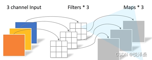
深度可分卷积(Depthwise Separable Convolution)=DW卷积+PW卷积(Pointwise Conv)
PW卷积是卷积核大小为1的普通卷积,理论上讲,普通卷积的计算量是CW+PW的8到9倍(此处默认输入矩阵和输出矩阵大小相同)
- 增加了两个人为设定的超参数α,β,α是Width Multiplier,用于控制卷积核个数,β是Resolution Multiplier,用于控制输入图像的大小
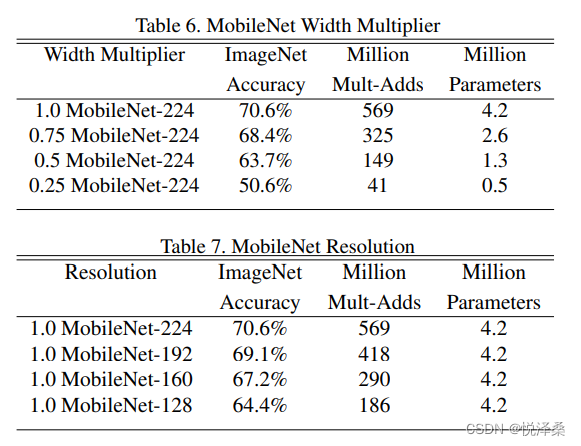
由此可见,可以通过适当的减小输入图像的大小,在准确率变化很小的情况下达到很少的参数量。但在实际使用中,DW卷积在大部分情况下没有起到作用,为解决这个问题,提出了MobileNetV2。V2准确率更高,模型更小。
V2网络亮点:
- Inverted Residuals(倒残差结构)
残差结构是先降维再升维,中间用3*3卷积,激活函数为ReLU:而倒残差结构是先升维再降维,中间用DW卷积,激活函数为ReLU6。ReLU6(x)=min(max(x,0),6),这使得激活函数的值不会超过6,更适合移动端设备,避免数值溢出带来的精度损失。倒残差结构如图,当stride=1且输入特征矩阵与输出特征矩阵的shape相同时才有shortcut连接。

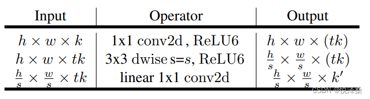
- Linear Bottlenecks
V2的倒残差结构的最后一层1*1卷积用的是线性的激活函数,因为ReLU会对低维特征信息造成大量损失。
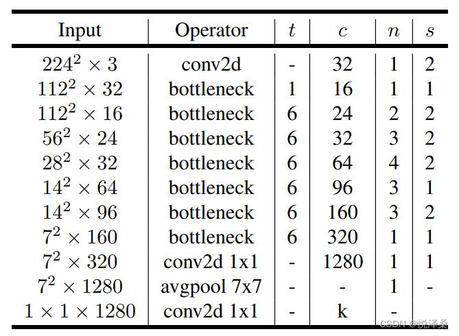
V2网络结构和参数如图,其中t是拓展音字,c是输出特征矩阵深度的channel,n是bottleneck的重复次数,s是第一层的步长,其他层的步长都是1:
1.2 基于PyTorch搭建MobileNet V2
代码链接:(colab)MobileNet
import torch
from torch import nn

# V2

def _make_divisible(ch,divisor=8,min_ch=None):
  if min_ch is None:
    min_ch = divisor
  new_ch = max(min_ch,int(ch*divisor/2)//divisor*divisor)
  # 确保向下取整时不会超过10%
  if new_ch<0.9*ch:
    new_ch+=diviser
  return new_ch


class ConvBNReLU(nn.Sequential):
  # group为1是普通卷积,group为输入特征矩阵的深度(in_channel)是DW卷积
  def __init__(self,in_channel,out_channel,kernel_size=3,stride=1,groups=1):
    padding = (kernel_size-1)//2
    super(ConvBNReLU,self).__init__(
        nn.Conv2d(in_channel,out_channel,kernel_size,stride,padding,groups=groups,bias=False),
        nn.BatchNorm2d(out_channel),
        nn.ReLU6(inplace=True)
    )

# 倒残差结构
class InvertedResidual(nn.Module):
  # expand_ratio即拓展因子t
  def __init__(self,in_channel,out_channel,stride,expand_ratio):
    super(InvertedResidual,self).__init__()
    # 隐层
    hidden_channel = in_channel*expand_ratio
    # 是否用shortcut
    self.use_shortcut = stride==1 and in_channel==out_channel

    layers = []
    if expand_ratio!=1:
      # 1*1 PW
      layers.append(ConvBNReLU(in_channel,hidden_channel,kernel_size=1))
    layers.extend([
      # 3*3 DW
      ConvBNReLU(hidden_channel,hidden_channel,stride=stride,groups=hidden_channel),
      # 1*1 PW(Linear)
      nn.Conv2d(hidden_channel,out_channel,kernel_size=1,bias=False),
      nn.BatchNorm2d(out_channel)
    ])

    self.conv = nn.Sequential(*layers)

  def forward(self,x):
    if self.use_shortcut:
      return x+self.conv(x)
    else:
      return self.conv(x)


class MobileNetV2(nn.Module):
  def __init__(self,num_classes=1000,alpha=1.0,round_nearest=8):
    super(MobileNetV2,self).__init__()
    block = InsertedResidual
    input_channel = _make_divisible(32*alpha,round_nearest)
    last_channel = _make_divisible(1280*alpha,round_nearest)

    inverted_residual_setting=[
      # t,c,n,s
      [1,16,1,1],
      [6,24,2,2],
      [6,32,3,2],
      [6,64,4,2],
      [6,96,3,1],
      [6,160,3,2],
      [6,320,1,1],
    ]

    features = []
    # conv1 layer
    features.append(ConvBNReLU(3,input_channel,stride=2))
    for t,c,n,s in inverted_residual_setting:
      output_channel = _make_divisible(c*alpha,round_nearest)
      for i in range(n):
        stride = s if i==0 else 1
        features.append(block(input_channel,output_channel,stride,expand_ratio=t))
        input_channel = output_channel

    features.append(ConvBNReLU(input_channel,last_channel,1))
    self.features = nn.Sequential(*features)

    # 分类器
    self.avgpool = nn.AdaptiveAvgPool2d((1,1))
    self.classifier = nn.Sequential(
      nn.Dropout(0.2),
      nn.Linear(last_channel,num_classes)
    )

    # 权重初始化
    for m in self.modules():
      if isinstance(m,nn.Conv2d):
        nn.init.kaiming_normal_(m.weight,mode='fan out')
        if m.bias is not None:
          nn.init.ones_(m.weight)
          nn.init.zeros_(m.bias)
      elif isinstance(m,nn.BatchNorm2d):
        nn.init.ones_(m.weight)
        nn.init.zeros_(m.bias)
      elif isinstance(m,nn.Linear):
        nn.init.normal_(m.weight,0,0.1)
        nn.init.zeros_(m.bias)

  def forward(self,x):
    x = self.features(x)
    x = self.avgpool(x)
    x = torch.flatten(x,1)
    x = self.classifier(x)
    return x
2 MobileNet V3
2.1 网络结构
在ImageNet分类任务中,V3比V2准确率更高,更高效,推理速度更快
V3网络亮点:
- 更新block(bneck)
在倒残差结构的基础上作了改动,加入了SE模块,更新了激活函数,当stride=1且input_c=output_c才有shortcut连接。
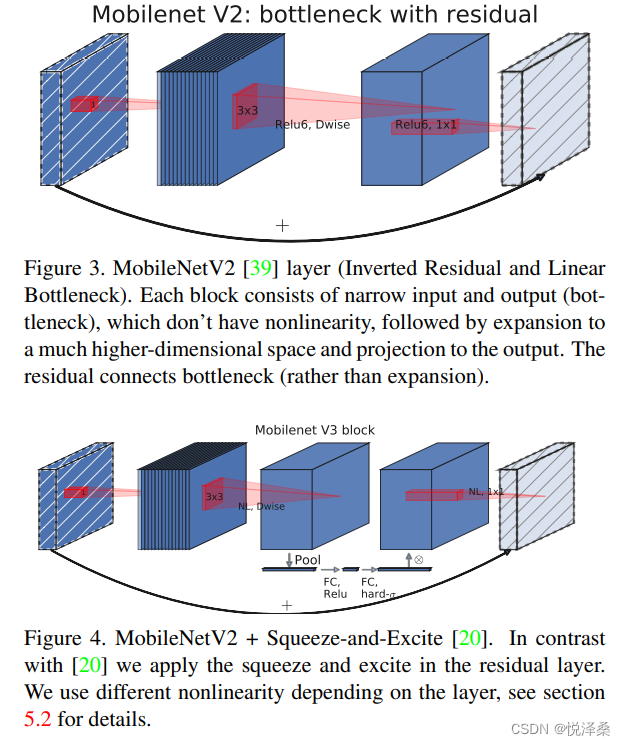
SE是通道注意力,对卷积得到的特征矩阵的每一个channel进行池化处理,再通过两个全连接层得到输出向量,第一个全连接层的结点个数为channel的四分之一,第二个全连接层的结点个数为channel
- 使用NAS搜索参数(Neural Architecture Search)
NAS是一种神经网络优化算法,先定义一组适用于我们网络的“构建块”再尝试以不同的方式组合这些“构建快”进行训练。通过这种试错方式,NAS算法最终能够确定哪一种“构建快”与哪一种网络配置可以得到最优结果。
卷积神经网络原理_怎样设计最优的卷积神经网络架构?| NAS原理剖析_LHZ5388015210的博客-CSDN博客
- 重新设计耗时层结构
减少了第一个卷积层的卷积核个数,由32个改为16个,并精简了Last Stage,减少了Last Stage的层数,保持了准确率,提升了速度。

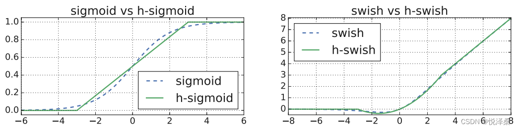
- 重新设计了激活函数
目前常用的激活函数是swish(x)=x*σ(x),其中σ(x)是sigmoid函数,但它计算和求导较复杂,对量化过程不友好,因此V3使用的是h-swish(x)=x*ReLU6(x+3)/6,其中ReLU6(x+3)/6是h-sigmoid。
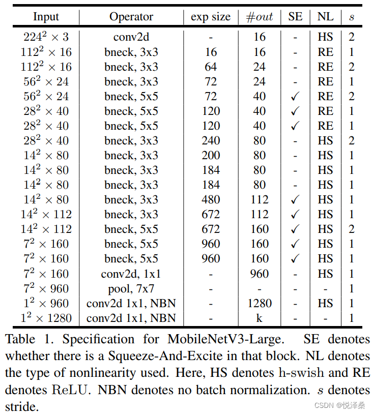
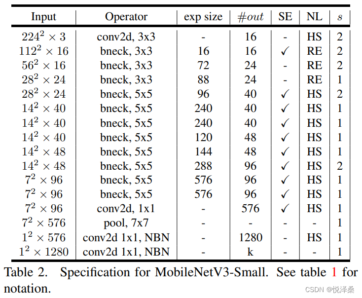
V3网络结构如下:
2.2 基于PyTorch搭建MobileNet V2
代码链接:(colab)MobileNet
import torch
from torch import nn,Tensor
from torch.nn import function as F

from typing import Callable,List,Optional
from functools import partial

# V3

def _make_divisible(ch,divisor=8,min_ch=None):
  if min_ch is None:
    min_ch = divisor
  new_ch = max(min_ch,int(ch*divisor/2)//divisor*divisor)
  # 确保向下取整时不会超过10%
  if new_ch<0.9*ch:
    new_ch+=diviser
  return new_ch


class ConvBNActivation(nn.Sequential):
  # group为1是普通卷积,group为输入特征矩阵的深度(in_channel)是DW卷积
  def __init__(self,
        in_planes:int,
        out_planes:int,
        kernel_size:int=3,
        stride:int=1,
        groups:int=1,
        norm_layer:Optional[Callable[...,nn.Module]]=None,
        activation_layer:Optional[Callable[...,nn.Module]]=None):
    padding = (kernel_size-1)//2
    if norm_layer is None:
      norm_layer = nn.BatchNorm2d
    if activation_layer is None:
      activation_layer = nn.ReLU6
    super(ConvBNActivation,self).__init__(nn.Conv2d(
                      in_channel=in_planes,
                      out_channel=out_planes,
                      kernel_size=kernel_size,
                      stride=stride,
                      padding=padding,
                      groups=groups,
                      bias=False),
                  norm_layer(out_planes),
                  activation_layer(inplace=True)))


# 注意力机制模块
class SqueezeExcitation(nn.Module):
  def __init__(self,input_c:int,squeeze_factor:int=4):
    super(SqueezeExcitation,self).__init__()
    squeeze_c = _make_divisible(input_c//squeeze_factor,8)
    self.fc1 = nn.Conv2d(input_c,squeeze_c,1)
    self.fc2 = nn.Conv2d(squeeze_c,input_c,1)

  def forward(self,x:Tensor) -> Tensor:
    scale = F.adaptive_avg_pool2d(x,output_size=(1,1))
    scale = self.fc1(scale)
    scale = F.relu(scale,inplace=True)
    scale = self.fc2(scale)
    scale = F.hardsigmoid(scale,inplace=True)
    return scale*x


# 倒残差结构
class InvertedResidualConfig:
  def __init__(self,input_c:int,
          kernel:int,
          expanded_c:int,
          out_c:int,
          use_se:bool,
          activation:str,
          stride:int,
          width_multi:float):
    self.input_c = self.adjust_channels(input_c,width_multi)
    self.kernel = kernel
    self.expanded_c = self.adjust_channels(expanded_c,width_multi)
    self.out_c = self.adjust_channels(out_c,width_multi)
    self.use_se = use_se
    self.use_hs = activation=="HS"
    self.stride = stride

  @staticmethod
  def adjust_channels(channels:int,width_multi:float):
    return _make_divisible(channels*width_multi,8)


# 倒残差结构
class InvertedResidual(nn.Module):
  def __init__(self,cnf:InvertedResidualConfig,
          norm_layer:Callable[...,nn.Module]):
    super(InvertedResidual,self).__init__()

    if cnf.stride not in [1,2]:
      raise ValueError("illegal stride value.")

    self.use_res_connect = (cnf.stride==1 and cnf.input_c==cnf.out_c)

    layers:List[nn.Module] = []
    activation_layer = nn.Hardswish if cnf.use_hs else nn.ReLU

    if cnf.expanded_c != cnf.input_c:
      layer.append(ConvBNActivation(cnf.input_c,
                    cnf.expanded_c,
                    kernel_size=1,
                    norm_layer=norm_layer,
                    activation_layer=activation_layer))
    # DW卷积
    layers.append(ConvBNActivation(cnf.expanded_c,
                  cnf.expanded_c,
                  kernel_size=cnf.kernel,
                  stride=cnf.stride,
                  groups=cnf.expanded_c,
                  norm_layer=norm_layer,
                  activation_layer=activation_layer))

    if cnf.use_se:
      layers.append(SqueezeExcitation(cnf.expanded_c))

    layers.append(ConvBNActivation(cnf.expanded_c,
                    cnf.out_c,
                    kernel_size=1,
                    norm_layer=norm_layer,
                    activation_layer=nn.Identity))

    self.block = nn.Sequential(*layers)
    self.out_channels = cnf.out_c

  def forward(self,x:Tensor) -> Tensor:
    result = self.block(x)
    if self.use_res_connect:
      result += x

    return result


class MobileNetV3(nn.Module):
  def __init__(self,
        inverted_residual_setting:List[InvertedResidualConfig],
        last_channel:int,
        num_classes:int=1000,
        block:Optional[Callable[...,nn.Module]]=None,
        norm_layer:Optional[Callable[...,nn.Module]]=None):
    super(MobileNetV3,self).__init__()

    if not inverted_residual_setting:
      raise ValueError("The inverted_residual_setting should not be empty.")
    elif not (isinstance(inverted_residual_setting,List) and
          all([isinstance(s,InvertedResidualConfig) for s in inverted_residual_setting])):
      raise TypeError("The inverted_residual_setting should be List[InvertedResidualConfig].")


    if block is None:
      block = InsertedResidual

    if norm_layer is None:
      norm_layer = partial(nn.BatchNorm2d,eps=0.001,momentum=0.01)

    layers:List[nn.Module] = []
    # 第一层
    firstconv_output_c = inverted_residual_setting[0].input_c
    layers.append(ConvBNActivation(3,firstconv_output_c,
                    kernel_size=3,
                    stride=2,
                    norm_layer=norm_layer,
                    activation_layer=nn.Hardswish))

    # 倒残差模块
    for cnf in inverted_residual_setting:
      layers.append(block(cnf,norm_layer))

    # 最后几层
    lastconv_input_c = inverted_residual_setting[-1].out_c
    lastconv_output_c = 6*lastconv_input_c
    layers.append(ConvBNActivation(lastconv_input_c,
                  lastconv_output_c,
                  kernel_size=1,
                  norm_layer=norm_layer,
                  avtivation_layer=nn.Hardswish))
    self.features = nn.Sequential(*layers)

    # 分类器
    self.avgpool = nn.AdaptiveAvgPool2d(1)
    self.classifier = nn.Sequential(
      nn.Linear(lastconv_output_c,last_channel),
      nn.Hardswish(inplace=True)
      nn.Dropout(p=0.2,inplace=True),
      nn.Linear(last_channel,num_classes)
    )

    # 权重初始化
    for m in self.modules():
      if isinstance(m,nn.Conv2d):
        nn.init.kaiming_normal_(m.weight,mode='fan out')
        if m.bias is not None:
          nn.init.zeros_(m.bias)
      elif isinstance(m,(nn.BatchNorm2d,nn.GroupNorm)):
        nn.init.ones_(m.weight)
        nn.init.zeros_(m.bias)
      elif isinstance(m,nn.Linear):
        nn.init.normal_(m.weight,0,0.01)
        nn.init.zeros_(m.bias)

  def _forward_impl(self,x:Tensor) -> Tensor:
    x = self.features(x)
    x = self.avgpool(x)
    x = torch.flatten(x,1)
    x = self.classifier(x)
    return x


def mobilenet_v3_large(num_classes:int=1000,reduced_tail:bool=False) -> MobileNetV3:
    width_multi = 1.0
    bneck_conf = partial(InvertedResidualConfig,width_multi=width_multi)
    adjust_channels = partial(InvertedResidualConfig.adjust_channels,width_multi=width_multi)

    reduce_divider = 2 if reduced_tail else 1

    inverted_residual_setting = [
        # input_c,kernel,expanded_c,out_c,use_se,activation,stride
        bneck_conf(16,3,16,16,False,"RE",1),
        bneck_conf(16,3,64,24,False,"RE",2),  # C1
        bneck_conf(24,3,72,24,False,"RE",1),
        bneck_conf(24,5,72,40,True,"RE",2), # C2
        bneck_conf(40,5,120,40,True,"RE",1),
        bneck_conf(40,5,120,40,True,"RE",1),
        bneck_conf(40,3,240,80,False,"HS",2), # C3
        bneck_conf(80,3,200,80,False,"HS",1),
        bneck_conf(80,3,184,80,False,"HS",1),
        bneck_conf(80,3,184,80,False,"HS",1),
        bneck_conf(80,3,480,112,True,"HS",1),
        bneck_conf(112,3,672,112,True,"HS",1),
        bneck_conf(112,5,672,160//reduce_divider,True,"HS",2),  # C4
        bneck_conf(160//reduce_divider,5,960//reduce_divider,160//reduce_divider,True,"HS",1),
        bneck_conf(160//reduce_divider,5,960//reduce_divider,160//reduce_divider,True,"HS",1)]
    last_channel = adjust_channels(1280//reduce_divider)  # C5

    return MobileNetV3(inverted_residual_setting=inverted_residual_setting,
              last_channel=last_channel,
              num_classes=num_classes)


def mobilenet_v3_small(num_classes:int=1000,reduced_tail:bool=False) -> MobileNetV3:

    width_multi = 1.0
    bneck_conf = partial(InvertedResidualConfig,width_multi=width_multi)
    adjust_channels = partial(InvertedResidualConfig.adjust_channels,width_multi=width_multi)

    reduce_divider = 2 if reduced_tail else 1

    inverted_residual_setting = [
        # input_c, kernel, expanded_c, out_c, use_se, activation, stride
        bneck_conf(16,3,16,16,True,"RE",2), # C1
        bneck_conf(16,3,72,24,False,"RE",2),  # C2
        bneck_conf(24,3,88,24,False,"RE",1),
        bneck_conf(24,5,96,40,True,"HS",2), # C3
        bneck_conf(40,5,240,40,True,"HS",1),
        bneck_conf(40,5,240,40,True,"HS",1),
        bneck_conf(40,5,120,48,True,"HS",1),
        bneck_conf(48,5,144,48,True,"HS",1),
        bneck_conf(48,5,288,96//reduce_divider,True,"HS",2),  # C4
        bneck_conf(96//reduce_divider,5,576//reduce_divider,96//reduce_divider,True,"HS",1),
        bneck_conf(96//reduce_divider,5,576//reduce_divider,96//reduce_divider,True,"HS",1)]
    last_channel = adjust_channels(1024//reduce_divider)  # C5

    return MobileNetV3(inverted_residual_setting=inverted_residual_setting,
              last_channel=last_channel,
              num_classes=num_classes)
3 SENet
相关链接:SENet
3.1 网络基本原理
为提升神经网络的性能,SENet(Squeeze-and-Excitation Networks)考虑从特征通道之间的关系入手,显示地表现出特征通道之间的依赖关系。SENet采用了“特征重标定”策略,通过学习的方式自动获取每个特征通道的重要程度,再按照重要程度来抑制用处不大的特征,突出有用的特征。
SENet有两个关键操作,一个是Squeeze,另一个是Excitation,因此得名。SENet的重要结构是SE模块,SE模块示意图如图所示:
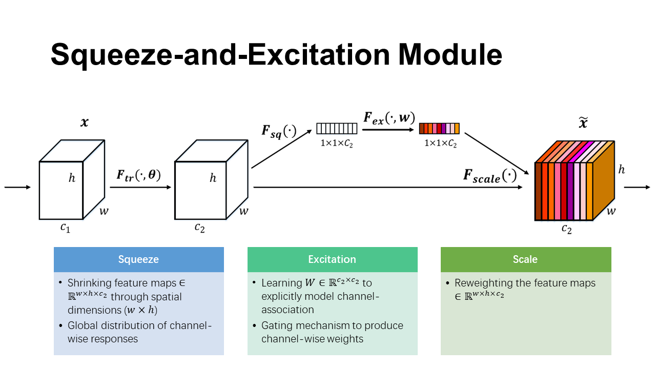
SE模块有三个操作:
- Squeeze操作:顺着空间维度进行特征压缩,将二维的特征通道转变为具有全局感受野的实数,并且要保证输出维度和输入特征通道数相匹配,使得靠近输入的层也能获得全局感受野。
- Excitation操作:类似于循环神经网络的门的机制,为每个特征通道生成权重,权重参数是通过学习得到的,能显示表现出特征通道间的相关性。
- Reweight操作:将得到的权重参数以乘法的形式加权到之前的特征上,实现在通道维度上的特征重标定。
SE模块具体结构如下,它可以嵌入到多种网络结构里发挥作用,容易部署,不需要引入新的函数或者层,有利于改善计算复杂度:
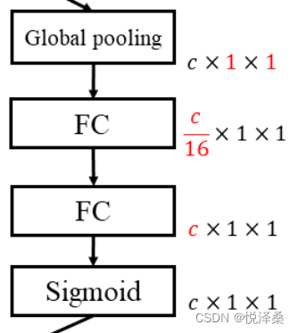
这里先使用全局平局池化作为Squeeze操作,再用两个FC组成Bottleneck结构进行Excitation。Excitation中先将特征维度降低到1/16,经过ReLU后再通过FC回到原来的维度,相比只用一个FC,这样处理有更多的非线性,并且能减少参数量。最后的Sigmoid使得最后能得到0~1的权重,再通过scale进行归一化,将权重加权到对应的特征上。
3.2 代码
import torch
import torch.nn as nn
import torch.nn.functional as F
import torchvision
import torchvision.transforms as transforms
import matplotlib.pyplot as plt
import numpy as np
import torch.optim as optim

class BasicBlock(nn.Module):
  def __init__(self,in_channels,out_channels,stride=1):
    super(BasicBlock,self).__init__()
    self.conv1 = nn.Conv2d(in_channels,out_channels,kernel_size=3,stride=stride,padding=1,bias=False)
    self.bn1 = nn.BatchNorm2d(out_channels)
    self.conv2 = nn.Conv2d(out_channels,out_channels,kernel_size=3,stride=1,padding=1,bias=False)
    self.bn2 = nn.BatchNorm2d(out_channels)

    # shortcut的输出维度和输出不一致时,用1*1的卷积来匹配维度
    self.shortcut = nn.Sequential()
    if stride!=1 or in_channels!=out_channels:
      self.shortcut = nn.Sequential(nn.Conv2d(in_channels,out_channels,kernel_size=1,stride=stride,bias=False),nn.BatchNorm2d(out_channels))

    # excitation
    self.fc1 = nn.Conv2d(out_channels,out_channels//16,kernel_size=1)
    self.fc2 = nn.Conv2d(out_channels//16,out_channels,kernel_size=1)

  #定义网络结构
  def forward(self, x):
    # 进行两次卷积得到压缩
    out = F.relu(self.bn1(self.conv1(x)))
    out = self.bn2(self.conv2(out))

    # Squeeze
    w = F.avg_pool2d(out,out.size(2))

    # Excitation
    w = F.relu(self.fc1(w))
    w = F.sigmoid(self.fc2(w))

    # 加权
    out = out*w
    # 加上浅层特征图
    out += self.shortcut(x)
    out = F.relu(out)
    return out


class SENet(nn.Module):
  def __init__(self):
    super(SENet,self).__init__()
    self.num_classes = 10
    self.in_channels = 64

    # 用64*3*3的卷积核
    self.conv1 = nn.Conv2d(3,64,kernel_size=3,stride=1,padding=1,bias=False)
    self.bn1 = nn.BatchNorm2d(64)
    # BasicBlock
    # 每个卷积层需要2个block块
    self.layer1 = self._make_layer(BasicBlock,64,2,stride=1)
    self.layer2 = self._make_layer(BasicBlock,128,2,stride=2)
    self.layer3 = self._make_layer(BasicBlock,256,2,stride=2)
    self.layer4 = self._make_layer(BasicBlock,512,2,stride=2)

    self.linear = nn.Linear(512,self.num_classes)

  #实现卷积
  #blocks为大layer中的残差块数
  #定义每一个layer有几个残差块,resnet18是2,2,2,2
  def _make_layer(self,block,out_channels,blocks,stride):
    strides = [stride]+[1]*(blocks-1)
    layers = []
    for stride in strides:
      layers.append(block(self.in_channels,out_channels,stride))
      self.in_channels = out_channels
    return nn.Sequential(*layers)

  def forward(self, x):
    out = F.relu(self.bn1(self.conv1(x)))
    out = self.layer1(out)
    out = self.layer2(out)
    out = self.layer3(out)
    out = self.layer4(out)
    out = F.avg_pool2d(out,4)
    out = out.view(out.size(0),-1)
    out = self.linear(out)
    return out
Part2 代码作业
2.1 2D卷积与3D卷积
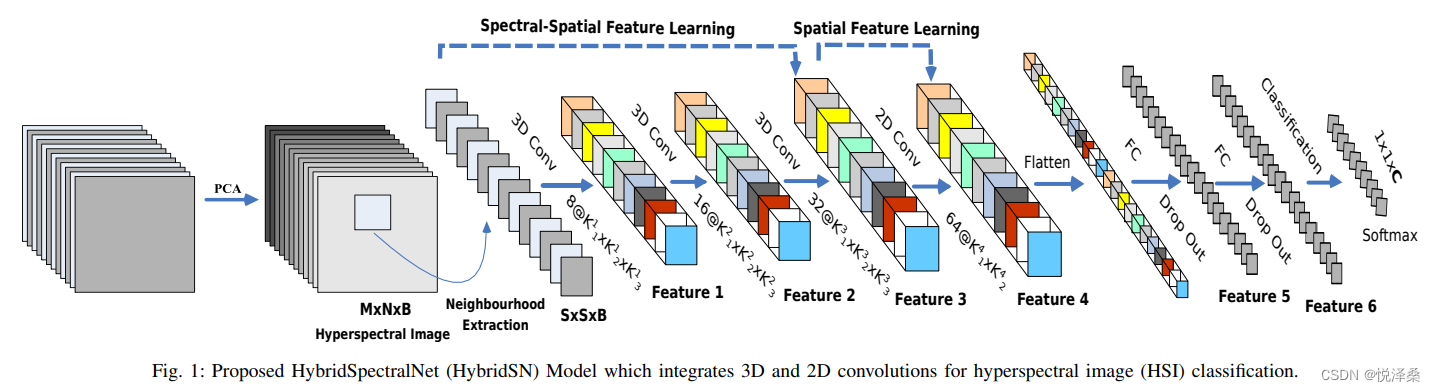
高光谱图像是三维立体数据,包含两个空间维度和一个光谱维度。对高光谱图像来说,二维卷积可以提取空间特征,但不能提取光谱特征,三维卷积可以同时提取空间特征和光谱特征,有利于提升分类准确率,但计算比二维卷积复杂。因此,《HybridSN: Exploring 3D-2D CNN Feature Hierarchy for Hyperspectral Image Classification》这篇论文结合二维卷积和三维卷积的优势,先使用三维卷积,再使用二维卷积,最后连接分类器,既能发挥三位卷积的优势,充分提取特征,也避免了三维卷积的过多使用导致模型复杂。
2.2 HybridSN
HybridSN结构如下:
代码链接:(colab)HybirdSN
网络部分代码补充:
class_num = 16

class HybridSN(nn.Module):

  def __init__(self,num_classes=16):
    super(HybridSN,self).__init__()
    self.conv1 = nn.Conv3d(1,8,(7,3,3))
    self.bn1=nn.BatchNorm3d(8)

    self.conv2 = nn.Conv3d(8,16,(5,3,3))
    self.bn2=nn.BatchNorm3d(16)

    self.conv3 = nn.Conv3d(16,32,(3,3,3))
    self.bn3=nn.BatchNorm3d(32)

    self.conv4 = nn.Conv2d(576,64,(3,3))
    self.bn4=nn.BatchNorm2d(64)

    self.drop = nn.Dropout(p=0.4)

    self.fc1 = nn.Linear(18496,256)
    self.fc2 = nn.Linear(256,128)
    self.fc3 = nn.Linear(128,num_classes)

    self.relu = nn.ReLU()

    # 论文里有加softmax,但本次实验下loss下降特别慢,因此没有使用
    self.softmax = nn.Softmax(dim=1)

  def forward(self,x):
    out = self.relu(self.bn1(self.conv1(x)))
    out = self.relu(self.bn2(self.conv2(out)))
    out = self.relu(self.bn3(self.conv3(out)))

    out = out.view(-1,out.shape[1]*out.shape[2],out.shape[3],out.shape[4])
    out = self.relu(self.bn4(self.conv4(out)))

    out = out.view(out.size(0),-1)
    out = self.fc1(out)
    out = self.drop(out)
    out = self.relu(out)
    out = self.fc2(out)
    out = self.drop(out)
    out = self.relu(out)
    out = self.fc3(out)
    # out = self.softmax(out)
    return out


# 随机输入,测试网络结构是否通
x = torch.randn(1,1,30,25,25)
net = HybridSN()
y = net(x)
print(y.shape)
相关资源下载:
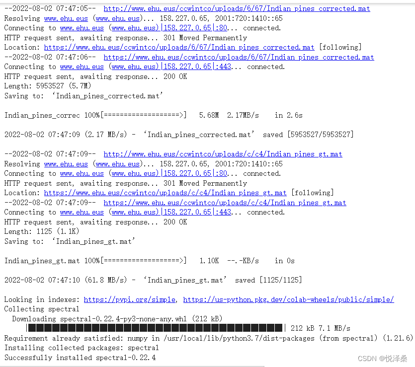
数据处理:

训练:
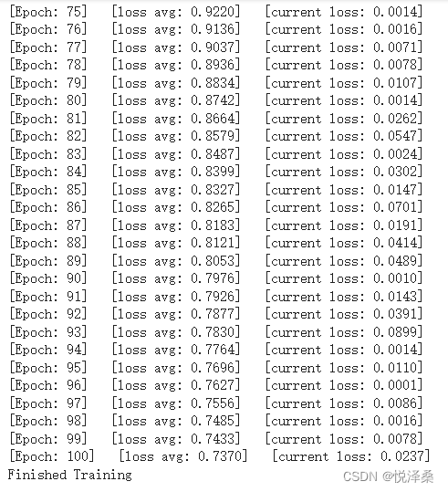
模型测试:

将分类结果写入文件:
第一次:
97.4536466477302 Kappa accuracy (%)
97.7669376693767 Overall accuracy (%)
94.13603236733026 Average accuracy (%)

                              precision    recall  f1-score   support

                     Alfalfa       0.95      0.93      0.94        41
                 Corn-notill       1.00      0.93      0.96      1285
                Corn-mintill       0.94      0.99      0.97       747
                        Corn       0.97      0.99      0.98       213
               Grass-pasture       0.94      0.98      0.96       435
                 Grass-trees       0.98      1.00      0.99       657
         Grass-pasture-mowed       0.92      0.96      0.94        25
               Hay-windrowed       0.99      1.00      1.00       430
                        Oats       0.75      0.50      0.60        18
              Soybean-notill       0.99      0.98      0.98       875
             Soybean-mintill       0.97      0.99      0.98      2210
               Soybean-clean       0.97      0.96      0.97       534
                       Wheat       0.99      0.96      0.98       185
                       Woods       1.00      0.99      1.00      1139
Buildings-Grass-Trees-Drives       0.98      0.97      0.98       347
          Stone-Steel-Towers       0.88      0.93      0.90        84

                    accuracy                           0.98      9225
                   macro avg       0.95      0.94      0.95      9225
                weighted avg       0.98      0.98      0.98      9225

[[  38    0    0    0    0    2    1    0    0    0    0    0    0    0
     0    0]
 [   1 1200   23    1    5    0    0    0    1    7   43    1    0    1
     1    1]
 [   0    0  740    0    3    0    0    0    0    0    0    3    1    0
     0    0]
 [   0    0    3  210    0    0    0    0    0    0    0    0    0    0
     0    0]
 [   0    0    2    0  428    1    0    0    0    0    4    0    0    0
     0    0]
 [   0    0    0    0    0  655    0    0    1    0    1    0    0    0
     0    0]
 [   0    0    0    0    1    0   24    0    0    0    0    0    0    0
     0    0]
 [   0    0    0    0    0    0    0  429    0    1    0    0    0    0
     0    0]
 [   0    0    8    0    0    1    0    0    9    0    0    0    0    0
     0    0]
 [   1    0    0    0    9    3    0    0    0  856    3    2    1    0
     0    0]
 [   0    2    6    0    1    4    0    1    0    1 2191    0    0    2
     2    0]
 [   0    0    2    4    0    0    0    0    1    1    0  514    0    0
     2   10]
 [   0    0    0    1    5    0    1    0    0    0    0    0  178    0
     0    0]
 [   0    1    0    0    0    0    0    1    0    0    2    1    0 1133
     1    0]
 [   0    0    0    0    1    0    0    1    0    0    8    1    0    0
   336    0]
 [   0    0    0    0    0    0    0    0    0    0    0    6    0    0
     0   78]]
第二次:
97.53900729242903 Kappa accuracy (%)
97.84281842818429 Overall accuracy (%)
95.58275885289382 Average accuracy (%)

                              precision    recall  f1-score   support

                     Alfalfa       0.95      0.88      0.91        41
                 Corn-notill       0.98      0.95      0.97      1285
                Corn-mintill       0.97      0.99      0.98       747
                        Corn       0.96      0.99      0.97       213
               Grass-pasture       1.00      0.96      0.98       435
                 Grass-trees       0.99      0.99      0.99       657
         Grass-pasture-mowed       1.00      1.00      1.00        25
               Hay-windrowed       0.99      1.00      0.99       430
                        Oats       0.82      0.78      0.80        18
              Soybean-notill       0.98      0.98      0.98       875
             Soybean-mintill       0.97      0.99      0.98      2210
               Soybean-clean       0.97      0.97      0.97       534
                       Wheat       0.97      0.98      0.98       185
                       Woods       0.99      1.00      0.99      1139
Buildings-Grass-Trees-Drives       0.99      0.95      0.97       347
          Stone-Steel-Towers       0.90      0.89      0.90        84

                    accuracy                           0.98      9225
                   macro avg       0.96      0.96      0.96      9225
                weighted avg       0.98      0.98      0.98      9225

[[  36    0    0    1    0    0    0    3    0    0    1    0    0    0
     0    0]
 [   2 1219    1    0    0    2    0    0    0    6   51    3    0    1
     0    0]
 [   0    1  741    5    0    0    0    0    0    0    0    0    0    0
     0    0]
 [   0    0    1  211    0    1    0    0    0    0    0    0    0    0
     0    0]
 [   0    1   12    0  416    0    0    0    0    1    4    1    0    0
     0    0]
 [   0    2    0    0    0  649    0    0    0    0    2    0    2    2
     0    0]
 [   0    0    0    0    0    0   25    0    0    0    0    0    0    0
     0    0]
 [   0    0    0    0    0    0    0  429    0    0    0    0    0    0
     0    1]
 [   0    0    3    0    0    0    0    0   14    0    0    0    1    0
     0    0]
 [   0    2    1    0    0    0    0    0    2  859    3    4    0    1
     2    1]
 [   0    3    1    0    1    3    0    0    0   10 2186    0    0    6
     0    0]
 [   0    0    3    3    0    0    0    1    1    0    0  519    0    0
     1    6]
 [   0    2    0    0    1    0    0    1    0    0    0    0  181    0
     0    0]
 [   0    4    0    0    0    0    0    0    0    0    0    0    0 1135
     0    0]
 [   0    6    0    0    0    0    0    0    0    1    5    0    2    2
   331    0]
 [   0    0    0    0    0    0    0    0    0    0    0    9    0    0
     0   75]]
可视化结果:
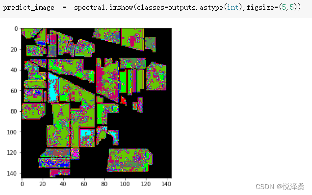
2.3 思考
① 测试了两次,发现这两次的结果不同,是因为网络中采用了dropout,每次使用该网络时丢弃的节点不相同,并且测试时没有将网络设置为eval。
② 进一步提升高光谱图像的分类性能,可以考虑加入SE注意力机制模块,或者引入Bottleneck结构调整特征的维度。