玩转深度学习——pytorch实现Lenet网络
什么是LeNet网络
LeNet,它是最早发布的卷积神经网络之一,因其在计算机视觉任务中的高效性能而受到广泛关注。 这个模型是由AT&T贝尔实验室的研究员Yann LeCun在1989年提出的(并以其命名),目的是识别图像 [LeCun et al., 1998]中的手写数字。 当时,Yann LeCun发表了第一篇通过反向传播成功训练卷积神经网络的研究,这项工作代表了十多年来神经网络研究开发的成果。论文文章地址,有兴趣可以深入阅读了解。
下面我们来看下LeNet(LeNet-5)的结构:LeNet网络结构十分简单,它由两个部分组成:一个是卷积编码器,另一个是全连接层密集块。其结构图如下:
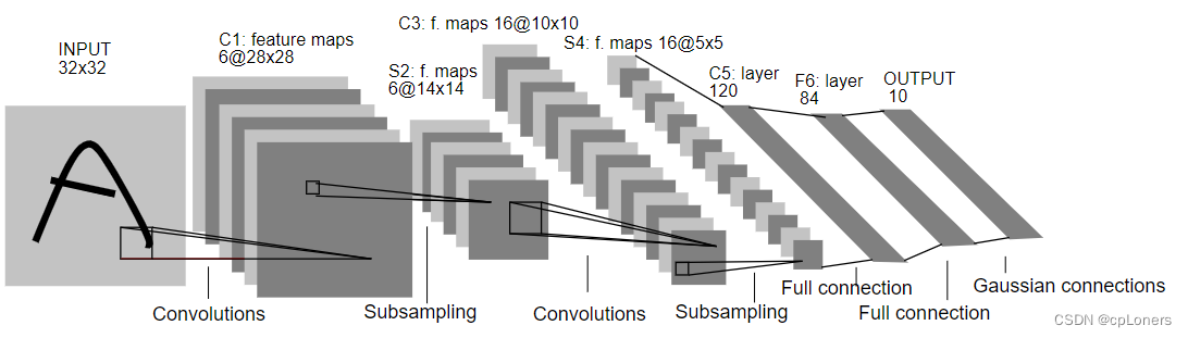
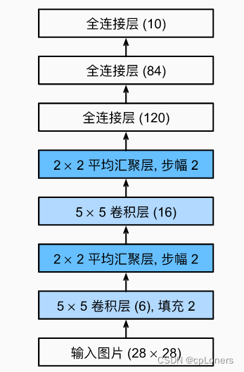
看不太懂,没关系,我们用流程图来画它的结构,这个可能会更好理解其结构:
LeNet网络pytorch实现
现在,我们对LeNet网络结构有了大致了解,接下来我们就使用pytorch来搭积木似的搭建LeNet网络,并且使用Fashion-MNIST数据集来测试下这个网络。(如果在搭建LeNet网络看不太懂,可以边看上面的流程图边来理解,注:Fashion-MNIST数据集的图片是单通道的,所以一开始输入的通道数为1)
import torch
from torch import nn
from torch.nn import init
import numpy as np
import sys
import torchvision
import torchvision.transforms as transforms
import time
import matplotlib.pyplot as plt
# 导入FashionMNIST数据集
mnist_train = torchvision.datasets.FashionMNIST(root='~/Datasets/FashionMNIST', train=True, download=True, transform=transforms.ToTensor())
mnist_test = torchvision.datasets.FashionMNIST(root='~/Datasets/FashionMNIST', train=False, download=True, transform=transforms.ToTensor())
# 处理数据集,把数据转换成张量,使数据可以输入下面我们搭建的网络
def load_data_fashion_mnist(mnist_train, mnist_test, batch_size):
if sys.platform.startswith('win'):
num_workers = 0
else:
num_workers = 4
train_data = torch.utils.data.DataLoader(mnist_train, batch_size=batch_size, shuffle=True, num_workers=num_workers)
test_data = torch.utils.data.DataLoader(mnist_test, batch_size=batch_size, shuffle=False, num_workers=num_workers)
return train_data, test_data
class LeNet(nn.Module):
def __init__(self):
super(LeNet, self).__init__()
self.conv = nn.Sequential(
nn.Conv2d(in_channels=1, out_channels=6, kernel_size=5), # in_channels, out_channels, kernel_size
nn.LeakyReLU(0.1),
nn.MaxPool2d(2, 2), # kernel_size, stride
nn.Conv2d(6, 16, 5),
nn.LeakyReLU(0.1),
nn.MaxPool2d(2, 2)
)
self.fc = nn.Sequential(
nn.Linear(16*4*4, 120),
nn.LeakyReLU(0.1),
nn.Linear(120, 84),
nn.ReLU(),
nn.Linear(84, 10)
)
def forward(self, img):
feature = self.conv(img)
output = self.fc(feature.view(img.shape[0], -1))
return output
# 测试准确率计算
def evaluate_accuracy(data_iter, net, device=None):
if device is None and isinstance(net, torch.nn.Module):
# 如果没指定device就使用net的device
device = list(net.parameters())[0].device
acc_sum, n = 0.0, 0
with torch.no_grad():
for X, y in data_iter:
net.eval() # 评估模式, 这会关闭dropout
acc_sum += (net(X.to(device)).argmax(dim=1) == y.to(device)).float().sum().cpu().item()
net.train() # 改回训练模式
n += y.shape[0]
return acc_sum / n
# 训练函数
def train(net, train_data, test_data, batch_size, optimizer, device, num_epochs):
net = net.to(device)
print("training on ", device)
loss_function = torch.nn.CrossEntropyLoss() # 定义损失函数(交叉熵损失函数)
ax = [] # 保存等会更新的epoch,loss,train_acc,test_acc,用于绘制动态折线图
ay1 = []
ay2 = []
ay3 = []
plt.ion()
# 开始训练
for epoch in range(num_epochs):
train_l_sum, train_acc_sum, n, batch_count, start = 0.0, 0.0, 0, 0, time.time() # 初始化参数
for X, y in train_data:
X = X.to(device) # 把参数导入GPU训练
y = y.to(device)
y_hat = net(X)
l = loss_function(y_hat, y) # 使用损失函数计算loss
optimizer.zero_grad()
l.backward() # 反向传播
optimizer.step()
train_l_sum += l.cpu().item()
train_acc_sum += (y_hat.argmax(dim=1) == y).sum().cpu().item()
n += y.shape[0]
batch_count += 1
test_acc = evaluate_accuracy(test_data, net) # 测试当个epoch的训练的网络
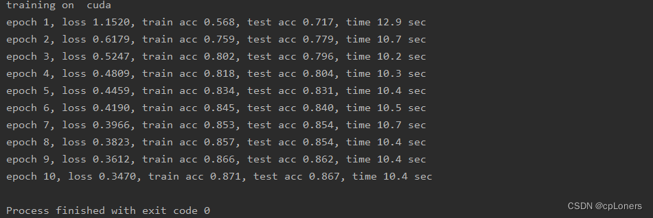
print('epoch %d, loss %.4f, train acc %.3f, test acc %.3f, time %.1f sec'
% (epoch + 1, train_l_sum / batch_count, train_acc_sum / n, test_acc, time.time() - start))
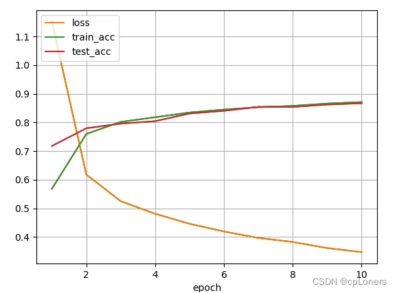
# 绘制动态折线图(如果不想绘制,可以删掉)
plt.clf() # 清除刷新前的图表,防止数据量过大消耗内存
ax.append(epoch + 1) # 追加x坐标值
ay1.append(train_l_sum / batch_count) # 追加y坐标值
ay2.append(train_acc_sum / n)
ay3.append(test_acc)
plt.plot(ax, ay1, 'g-')
plt.plot(ax, ay2, 'r-')
plt.plot(ax, ay3, '-')
plt.ylabel("epoch")
plt.plot(ax, ay1, label="loss") # 在绘图函数添加一个属性label
plt.plot(ax, ay2, label="train_acc")
plt.plot(ax, ay3, label="test_acc")
plt.legend(loc=2) # 添加图例,loc为图例位置,1为右上角,2为左上角,3为左下角,4为右下角
plt.grid() # 添加网格
plt.pause(5) # 设置暂停时间,太快图表无法正常显示
plt.ioff() # 关闭画图的窗口,即关闭交互模式
plt.show() # 显示图片,防止闪退
if __name__ == '__main__':
batch_size = 256 # 批量数大小
train_data, test_data = load_data_fashion_mnist(mnist_train, mnist_test, batch_size)
device = torch.device('cuda' if torch.cuda.is_available() else 'cpu') # 使用GPU,如果没有则使用CPU
net = LeNet() # 导入我们搭建好的网络
lr, num_epochs = 0.001, 10
optimizer = torch.optim.Adam(net.parameters(), lr=lr) # 优化函数
train(net, train_data, test_data, batch_size, optimizer, device, num_epochs)
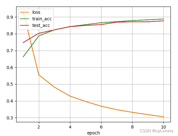
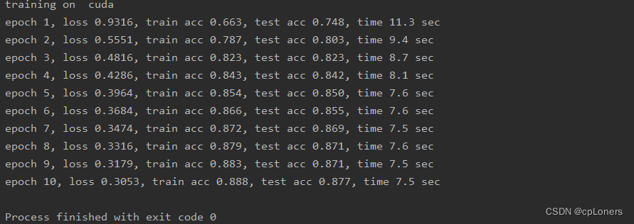
运行结果:
改进LeNet网络
在改进LeNet网络前,我在前面说了一下搭积木似的搭建LeNet,其实深度学习的网络搭建确实像在搭积木,如果我们把网络中的每个层,卷积块当成一块特定形状的积木块,在构建深度网络时,这不就像在搭积木了吗。
增加卷积层
上面的LeNet使用的卷积核大小为5 × \times × 5卷积块,我们尝试把它换成两个卷积核大小为5 × \times × 5卷积块,看看会发生什么
代码:
import torch
from torch import nn
from torch.nn import init
import numpy as np
import sys
import torchvision
import torchvision.transforms as transforms
import time
import matplotlib.pyplot as plt


# 导入FashionMNIST数据集
mnist_train = torchvision.datasets.FashionMNIST(root='~/Datasets/FashionMNIST', train=True, download=True, transform=transforms.ToTensor())
mnist_test = torchvision.datasets.FashionMNIST(root='~/Datasets/FashionMNIST', train=False, download=True, transform=transforms.ToTensor())


# 处理数据集,把数据转换成张量,使数据可以输入下面我们搭建的网络
def load_data_fashion_mnist(mnist_train, mnist_test, batch_size):
    if sys.platform.startswith('win'):
        num_workers = 0
    else:
        num_workers = 4
    train_data = torch.utils.data.DataLoader(mnist_train, batch_size=batch_size, shuffle=True, num_workers=num_workers)
    test_data = torch.utils.data.DataLoader(mnist_test, batch_size=batch_size, shuffle=False, num_workers=num_workers)
    return train_data, test_data


class LeNet(nn.Module):
    def __init__(self):
        super(LeNet, self).__init__()
        self.conv = nn.Sequential(
            nn.Conv2d(in_channels=1, out_channels=2, kernel_size=3), # in_channels, out_channels, kernel_size
            nn.LeakyReLU(0.1),
            nn.Conv2d(in_channels=2, out_channels=4, kernel_size=3),  # in_channels, out_channels, kernel_size
            nn.LeakyReLU(0.1),
            nn.MaxPool2d(2, 2), # kernel_size, stride
            nn.Conv2d(in_channels=4, out_channels=8, kernel_size=3),  # in_channels, out_channels, kernel_size
            nn.LeakyReLU(0.1),
            nn.Conv2d(in_channels=8, out_channels=16, kernel_size=3),  # in_channels, out_channels, kernel_size
            nn.LeakyReLU(0.1),
            nn.MaxPool2d(2, 2)
        )
        # self.avg_pool = nn.AdaptiveAvgPool2d(1)
        # self.se = nn.Sequential(
        #     nn.Linear(16, 2),
        #     nn.ReLU(inplace=True),
        #     nn.Linear(2, 16),
        #     nn.Sigmoid()
        # )
        self.fc = nn.Sequential(
            nn.Linear(16*4*4, 120),
            nn.LeakyReLU(0.1),
            nn.Linear(120, 84),
            nn.ReLU(),
            nn.Linear(84, 10)
        )

    def forward(self, img):
        feature = self.conv(img)
        # b, c, _, _ = feature.size()
        #
        # y = self.avg_pool(feature).view(b, c)
        # y = self.se(y).view(b, c, 1, 1)
        # feature = feature * y

        output = self.fc(feature.view(img.shape[0], -1))
        return output


# 测试准确率计算
def evaluate_accuracy(data_iter, net, device=None):
    if device is None and isinstance(net, torch.nn.Module):
        # 如果没指定device就使用net的device
        device = list(net.parameters())[0].device
    acc_sum, n = 0.0, 0
    with torch.no_grad():
        for X, y in data_iter:
            net.eval()  # 评估模式, 这会关闭dropout
            acc_sum += (net(X.to(device)).argmax(dim=1) == y.to(device)).float().sum().cpu().item()
            net.train()  # 改回训练模式
            n += y.shape[0]
    return acc_sum / n


# 训练函数
def train(net, train_data, test_data, batch_size, optimizer, device, num_epochs):
    net = net.to(device)
    print("training on ", device)
    loss_function = torch.nn.CrossEntropyLoss()   # 定义损失函数(交叉熵损失函数)
    ax = []  # 保存等会更新的epoch,loss,train_acc,test_acc,用于绘制动态折线图
    ay1 = []
    ay2 = []
    ay3 = []
    plt.ion()
    # 开始训练
    for epoch in range(num_epochs):
        train_l_sum, train_acc_sum, n, batch_count, start = 0.0, 0.0, 0, 0, time.time()  # 初始化参数
        for X, y in train_data:
            X = X.to(device)      # 把参数导入GPU训练
            y = y.to(device)
            y_hat = net(X)
            l = loss_function(y_hat, y)   # 使用损失函数计算loss
            optimizer.zero_grad()
            l.backward()   # 反向传播
            optimizer.step()
            train_l_sum += l.cpu().item()
            train_acc_sum += (y_hat.argmax(dim=1) == y).sum().cpu().item()
            n += y.shape[0]
            batch_count += 1
        test_acc = evaluate_accuracy(test_data, net)  # 测试当个epoch的训练的网络
        print('epoch %d, loss %.4f, train acc %.3f, test acc %.3f, time %.1f sec'
              % (epoch + 1, train_l_sum / batch_count, train_acc_sum / n, test_acc, time.time() - start))
        # 绘制动态折线图(如果不想绘制,可以删掉)
        plt.clf()  # 清除刷新前的图表,防止数据量过大消耗内存
        ax.append(epoch + 1)  # 追加x坐标值
        ay1.append(train_l_sum / batch_count)  # 追加y坐标值
        ay2.append(train_acc_sum / n)
        ay3.append(test_acc)
        plt.plot(ax, ay1, 'g-')
        plt.plot(ax, ay2, 'r-')
        plt.plot(ax, ay3, '-')
        plt.xlabel("epoch")
        plt.plot(ax, ay1, label="loss")  # 在绘图函数添加一个属性label
        plt.plot(ax, ay2, label="train_acc")
        plt.plot(ax, ay3, label="test_acc")
        plt.legend(loc=2)  # 添加图例,loc为图例位置,1为右上角,2为左上角,3为左下角,4为右下角
        plt.grid()   # 添加网格
        plt.pause(5)  # 设置暂停时间,太快图表无法正常显示
        plt.ioff()  # 关闭画图的窗口,即关闭交互模式
    plt.show()  # 显示图片,防止闪退


if __name__ == '__main__':
    batch_size = 256   # 批量数大小
    train_data, test_data = load_data_fashion_mnist(mnist_train, mnist_test, batch_size)
    device = torch.device('cuda' if torch.cuda.is_available() else 'cpu')  # 使用GPU,如果没有则使用CPU
    net = LeNet()    # 导入我们搭建好的网络
    lr, num_epochs = 0.001, 10
    optimizer = torch.optim.Adam(net.parameters(), lr=lr)  # 优化函数
    train(net, train_data, test_data, batch_size, optimizer, device, num_epochs)
这个改动看上去好像没有原来的结果,但这并不表示5 × \times × 5的卷积核就比两个3 × \times × 3好喔,原因是我们还没有进行大量的调参和训练的num_epochs不够。所以有兴趣的可以取尝试把num_epochs调大一下看看,比如20,50,100…,其他参数的调整我们会在下小节讲。
尝试修改一些超参数(开始炼丹)
我们常常在学习深度学习时会听到炼丹一词,其实这就是形容我们在确定一个网络框架后,在训练时不断调整一下超参数,使网络能发挥出其最好的性能。所以,这一过程常被调侃成在炼丹。确实也很形象。因为神经网络(特别是很深的网络)往往有大量的参数需要我们去手动调整为最优的参数。一般经常调整的参数有卷积核大小(每一个卷积块的卷积核大小的改变都有可能会影响最后的结果),步幅大小,学习率等等。上面我们已经尝试了改变卷积大小的。所以下面我们就不在一一展示其他超参数的修改了。
说到这里,是否会有一个疑问,既然这些超参数调整这么麻烦且耗费时间,那我能不能让它自己自动调参数,达到一个最优参数呢?确实是可以的。Barret Zoph在2016年就提出了Neural architecture search with reinforcement learning。 在Neurual Architecture Search的过程中,Barret Zoph使用一个RNN控制器来生成神经网络的一些超参数,对于神经网络的某一层来说,RNN预测它的过滤器高度、过滤器宽度、步幅高度、步幅宽度以及一层和重复的过滤器数量。每个预测都通过softmax分类器进行计算,并且将其输出送入下一个时间步的输入,重复这一过程。当神经网络的层数超过一个指定值时便停止继续生成。每当控制器RNN生成一个结构时,都要对这个结构进行训练以获得精度值,利用这个精度值便可以更新RNN。从而获得最优的超参数。这里的RNN是一个比LeNet还复杂的网络,后面我们会学到。有兴趣的可以去看看原论文了解下。