机器学习领域中所谓的降维就是指采用某种映射方法,将原高维空间中的数据点映射到低维度的空间中。降维的本质是学习一个映射函数 f : x->y,其中x是原始数据点的表达,目前最多使用向量表达形式。 y是数据点映射后的低维向量表达,通常y的维度小于x的维度(当然提高维度也是可以的)。f可能是显式的或隐式的、线性的或非线性的。
目前大部分降维算法处理向量表达的数据,也有一些降维算法处理高阶张量表达的数据。之所以使用降维后的数据表示是因为在原始的高维空间中,包含有冗余信息以及噪音信息,在实际应用例如图像识别中造成了误差,降低了准确率;而通过降维,我们希望减少 冗余信息 所造成的误差,提高识别(或其他应用)的精度。又或者希望通过降维算法来寻找数据内部的本质结构特征。
在很多算法中,降维算法成为了数据预处理的一部分,如PCA。事实上,有一些算法如果没有降维预处理,其实是很难得到很好的效果的。
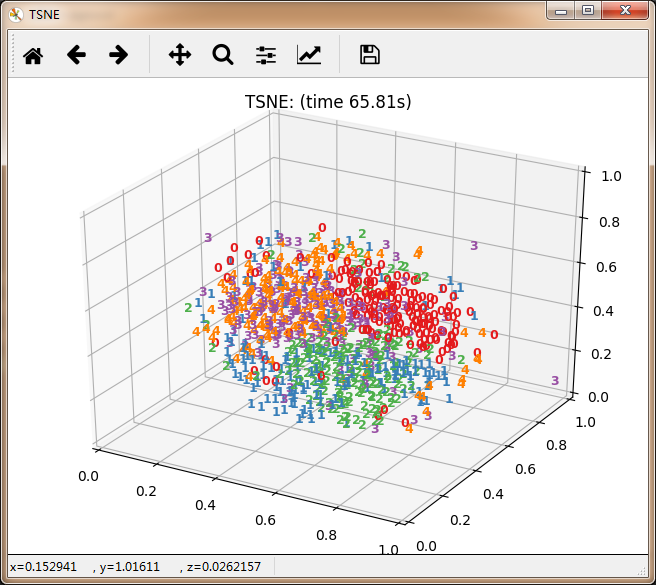
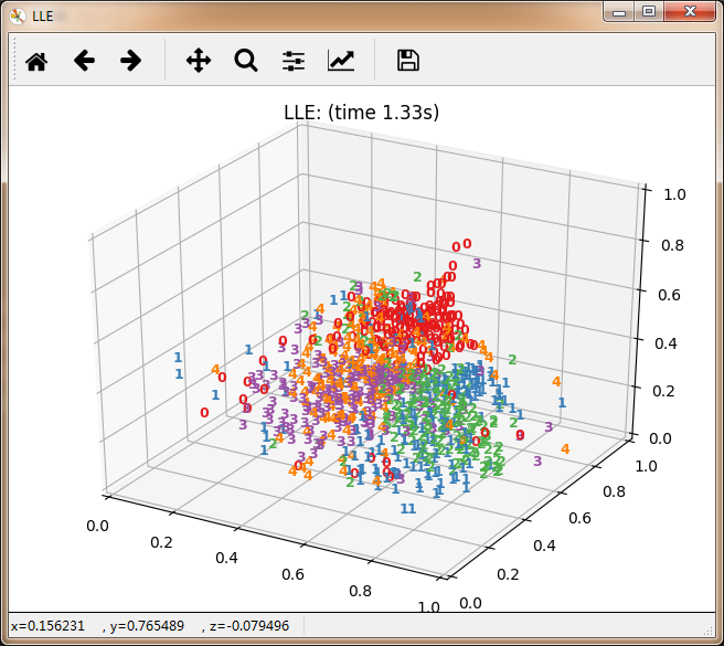
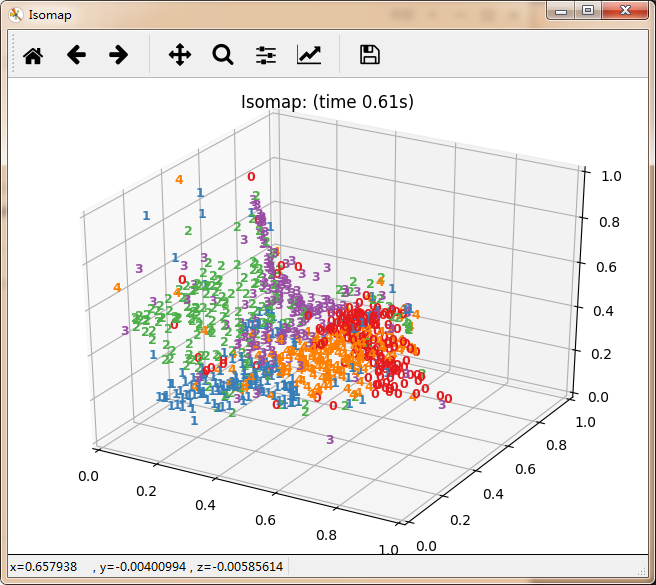
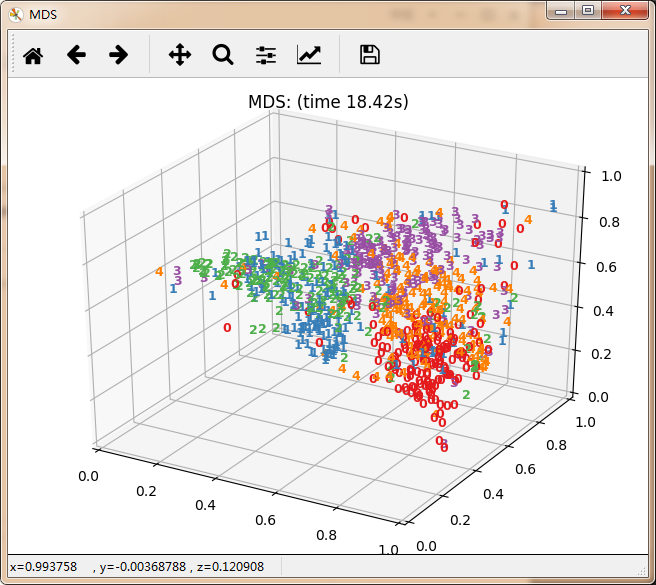
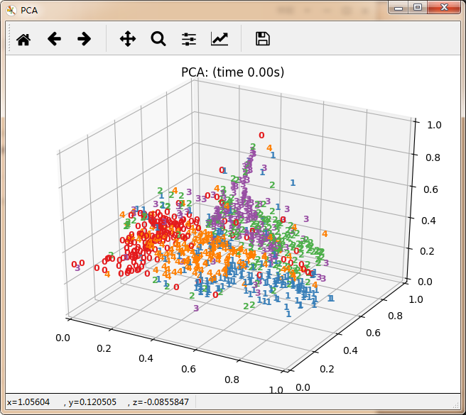
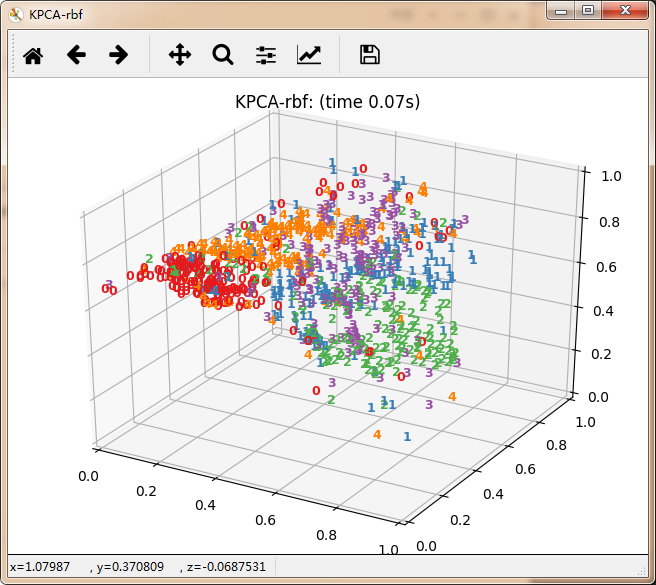
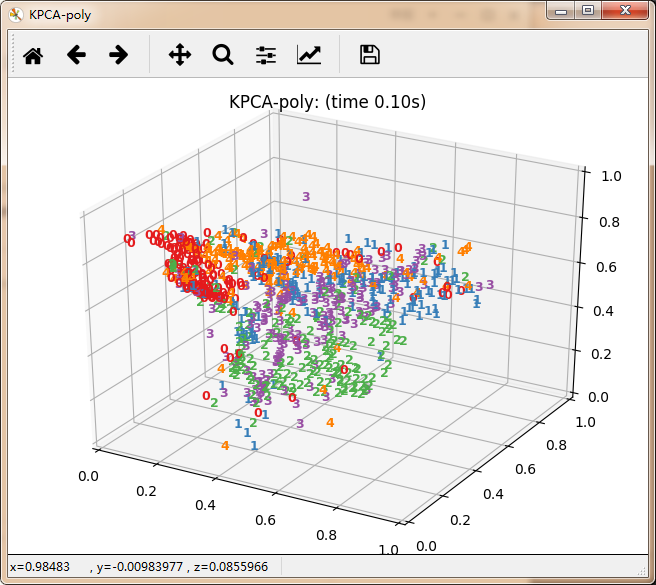
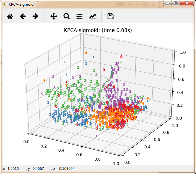
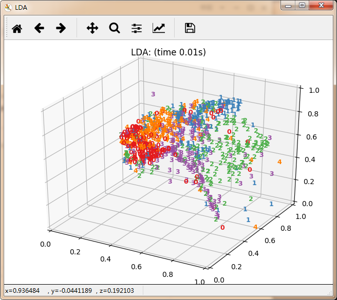
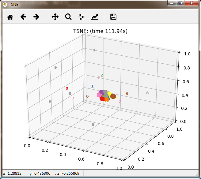
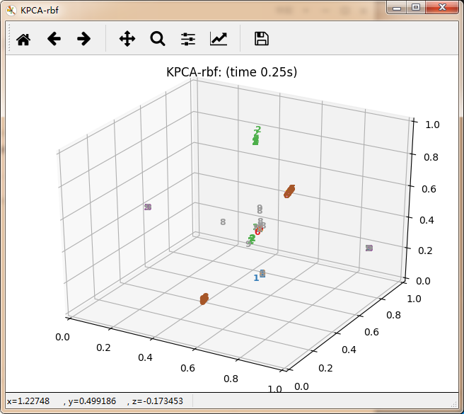
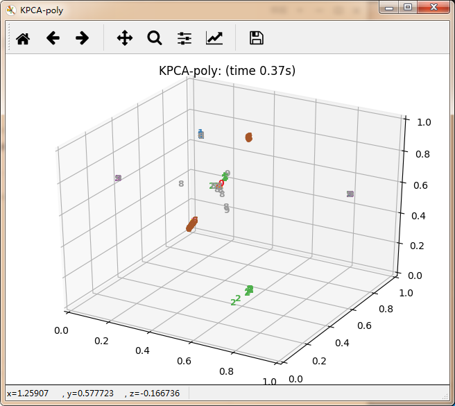
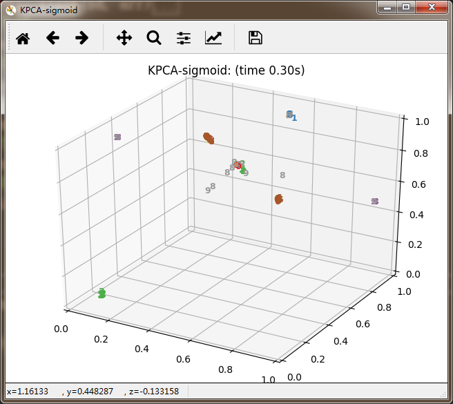
数据降维主要分为线性方法与非线性方法。其中线性方法主要有无监督PCA、有监督LDA。非线性方法有以保留局部特征为代表的基于重建权值的LLE、基于邻接图的拉普拉斯特征映射等。还有保留全局特征为代表的基于核KPCA、基于距离保持的MDS(欧式距离)极其扩展算法Isomap(测地线距离)。以及定义数据的局部和全局结构之间的软边界的t-SNE。每种算法都有其适用的应用领域,具体使用那种算法极其参数设置都需要根据具体情况进行确认。
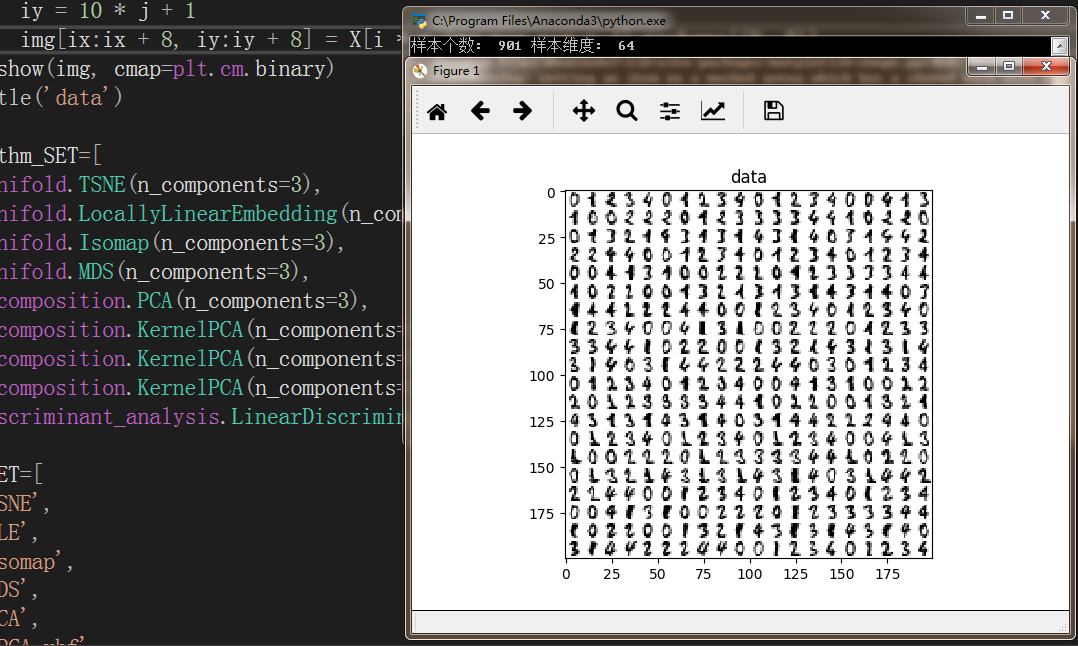
下面以digits数字图像集为例来对比一下各大降维算法。不过也不能完全说明问题,因为有些算法并不适合处理此类数据,
from time import time
import numpy as np
import matplotlib.pyplot as plt
from matplotlib import offsetbox
from sklearn import manifold, datasets, decomposition, ensemble,discriminant_analysis, random_projection
from mpl_toolkits.mplot3d import Axes3D
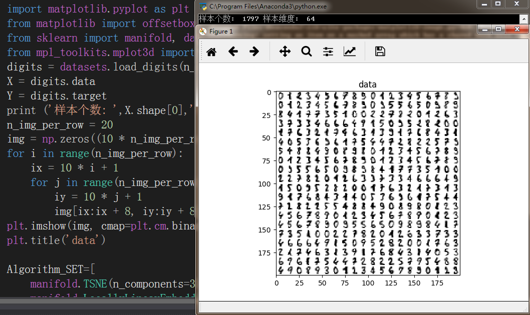
digits = datasets.load_digits(n_class=5)
X = digits.data
Y = digits.target
print ('样本个数: ',X.shape[0],'样本维度: ',X.shape[1])
n_img_per_row = 20
img = np.zeros((10 * n_img_per_row, 10 * n_img_per_row))
for i in range(n_img_per_row):
ix = 10 * i + 1
for j in range(n_img_per_row):
iy = 10 * j + 1
img[ix:ix + 8, iy:iy + 8] = X[i * n_img_per_row + j].reshape((8, 8))
plt.imshow(img, cmap=plt.cm.binary)
plt.title('data')
Algorithm_SET=[
manifold.TSNE(n_components=3),
manifold.LocallyLinearEmbedding(n_components=3),
manifold.Isomap(n_components=3),
manifold.MDS(n_components=3),
decomposition.PCA(n_components=3),
decomposition.KernelPCA(n_components=3,kernel='rbf'),
decomposition.KernelPCA(n_components=3,kernel='poly'),
decomposition.KernelPCA(n_components=3,kernel='sigmoid'),
discriminant_analysis.LinearDiscriminantAnalysis(n_components=3)
]
Name_SET=[
'TSNE',
'LLE',
'Isomap',
'MDS',
'PCA',
'KPCA-rbf',
'KPCA-poly',
'KPCA-sigmoid',
'LDA'
]
for i,Algorithm in enumerate(Algorithm_SET):
t0 = time()
X = Algorithm.fit_transform(X,Y)
#坐标缩放到[0,1]区间
x_min, x_max = np.min(X,axis=0), np.max(X,axis=0)
X = (X - x_min) / (x_max - x_min)
title = Name_SET[i]+": (time %.2fs)" %(time() - t0)
fig = plt.figure(Name_SET[i])
ax = Axes3D(fig)
for j in range(X.shape[0]):
ax.text(X[j, 0], X[j, 1], X[j,2],str(Y[j]),color=plt.cm.Set1((Y[j]+1) / 10.),fontdict={'weight': 'bold', 'size': 9})
plt.title(title)
plt.show()
再看10个分类的:
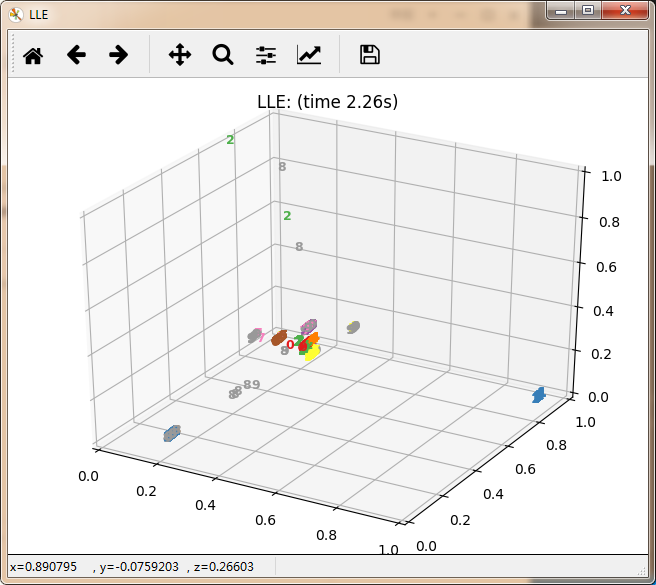
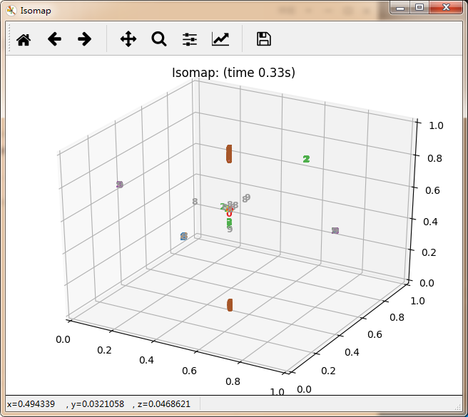
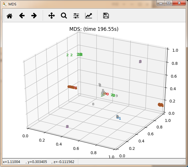
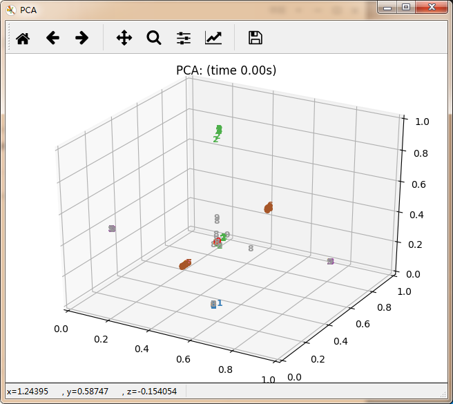
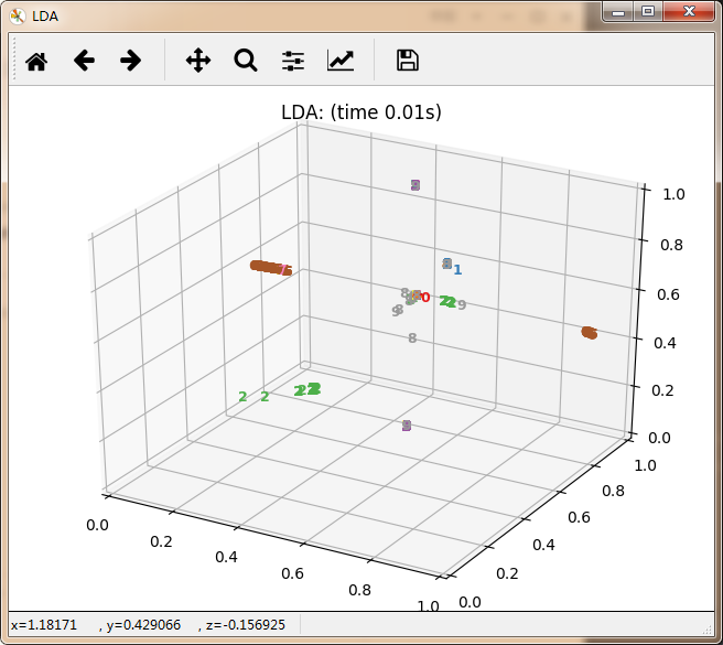
感觉除了时间复杂度炸裂的t_SNE,其他的都仿佛失了智一样。
至此,机器学习部分就先告一段落了,总体来说还是蛮难搞的,虽然强大的sklearn库可以提供各种API以及测试数据,不过若想深入了解其中的原理,必须要自己一步一步的推导,一步一步的实现。比如这个:
接下来学习Deep Learning还会面临更高的挑战,我只能说,祝大家身体健康吧- -再见!
