写在前面

参考的是https://zh.d2l.ai/index.html

一、实验目的与要求

(1)利用基于深度学习的特征自动学习方法完成图像特征提取的实验方案的设计。
(2)编程并利用相关软件完成实验测试，得到实验结果。
(3)通过对实验数据的分析、整理，得出实验结论，培养学生创新思维和编写实验报告的能力，以及处理一般工程设计技术问题的初步能力及实事求是的科学态度。
(4)利用实验更加直观、方便和易于操作的优势，提高学生学习兴趣，让学生自主发挥设计和实施实验发挥出学生潜在的积极性和创造性。

二、实验内容

(1)采用已经学过的深度特征提取方法，如卷积神经网络( CNN )等实现图像特征提取和学习的任务。
(2)分析比较深度学习方法的优缺点。

三、实验设备与环境

Windows11系统、Anaconda3、Pycharm Community、Jupyter Notebook、Scikit-learn库、TensorFlow深度学习框架、Pytorch深度学习框架

四、设计正文

（包括分析与设计思路、各模块流程图以及带注释的主要算法源码，若有改进或者创新，请描述清楚，并在实验结果分析中对比改进前后的结果并进行分析）

4.1 分析与设计思路

卷积神经网络是含有卷积层的神经网络，常用来处理图像数据。
卷积运算用星号表示。卷积的第一个参数为输入，第二个参数被称为核函数。输出为特征映射。将一张二维的图像 $I$ 作为输入，用一个二维的核 $K$ ，则：
$S(i,j)=(I\ast K)(i,j)=\sum_m\sum_n I(m,n)K(i-m,j-n)$
实际上，在深度学习领域的“卷积”都是指互相关运算。二维卷积层输出的二维数组可以看做输入在空间维度上某一级的表征（特征图）。假设输入的形状是 $n_h*n_w$ ，卷积核窗口形状是 $k_h*k_w$ ，在步长为1的情况下，则输出形状是 $n_h-k_h+1)(n_w-k_w+1)$ 。
填充(padding)是指在输入高和宽的两侧填充元素（0元素）。如果在高的两侧填充 $p_h$ 行，在宽的两侧填充 $p_w$ 列，则输出形状将变成：
$n_h-k_h+p_h+1)(n_w-k_w+p_w+1)$
使用更大的步长时，若高上步长 $s_h$ ，宽上步长 $s_w$ ，则输出形状为：
$\lfloor (n_h-k_h+p_h+1)/s_h\rfloor\lfloor(n_w-k_w+p_w+1)/s_w\rfloor$
对于彩色图像，可以有多个输入通道和多个输出通道。在做互相关运算时，每个输出通道上的结果由卷积核在该输出通道上的核数组与整个输入数组计算而来。
同卷积层一样，池化层每次对输入数据有一个固定形状窗口（池化窗口）。不同于卷积层内计算输入和核的互相关性，池化层直接计算池化窗口内元素的最大值或平均值。同卷积层一样，池化层也可以在输入的高和宽的两侧填充并调整窗口的移动步幅改变输出形状。在处理多通道输入数据时，池化层对每个输入通道分别池化，而不像卷积层那样将各通道输入按通道相加。所以池化层输出通道数和输入通道数相等。
在本次实验中，使用经典的LeNet卷积神经网络。LeNet分为卷积层块和全连接层块两个部分。卷积层块的基本单位是卷积层后接最大池化层。卷积层用来识别图像里的空间模式如线条或物体局部，之后的最大池化层用来降低卷积层对位置的敏感性。卷积层块由两个这样的基本单位重复堆叠构成，在卷积层块中每个卷积层使用5*5的窗口，并在输出上使用sigmoid激活函数。第一个卷积层输出通道数为6，第二个卷积层输出通道数增加到16。卷积层和两个最大池化层窗口均为2*2，且步长为2。所以池化窗口每次滑动所覆盖区域互不重叠。在将卷积层块的输出送入全连接层块前，全连接层块会将小批量中每个样本变平。全连接层输入性状将变成二维，第一维是小批量中的样本，第二维是每个样本变平后的向量表示，且向量长度为通道高宽的积。全连接层块含3个全连接层，输出个数分别是120、84、10，其中10位输出的类别个数。
LeNet卷积神经网络的整体流程如下:
在这里插入图片描述
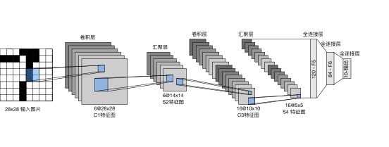
在本次实验中，使用经典的Fashion-MNIST数据集进行测试。

4.2 主要算法源码

import os
os.environ["KMP_DUPLICATE_LIB_OK"]="TRUE"
import torch
from torch import nn
from d2l import torch as d2l
net = nn.Sequential(
    nn.Conv2d(1, 6, kernel_size=5, padding=2), nn.Sigmoid(),#卷积
    nn.AvgPool2d(kernel_size=2, stride=2),#平均池化
    nn.Conv2d(6, 16, kernel_size=5), nn.Sigmoid(),#卷积
    nn.AvgPool2d(kernel_size=2, stride=2),#平均池化
    nn.Flatten(),#展平
    nn.Linear(16 * 5 * 5, 120), nn.Sigmoid(),#全连接
    nn.Linear(120, 84), nn.Sigmoid(),#全连接
    nn.Linear(84, 10))#全连接
X = torch.rand(size=(1, 1, 28, 28), dtype=torch.float32)#随机初始化种子
for layer in net:
    X = layer(X)
    print(layer.__class__.__name__,'output shape: \t',X.shape)
batch_size = 256
train_iter, test_iter = d2l.load_data_fashion_mnist(batch_size=batch_size)#读取训练集并batch
def evaluate_accuracy_gpu(net, data_iter, device=None): #@save
    """使用GPU计算模型在数据集上的精度"""
    if isinstance(net, nn.Module):
        net.eval()  # 设置为评估模式
        if not device:
            device = next(iter(net.parameters())).device
    # 正确预测的数量，总预测的数量
    metric = d2l.Accumulator(2)
    with torch.no_grad():
        for X, y in data_iter:
            if isinstance(X, list):
                # BERT微调
                X = [x.to(device) for x in X]
            else:
                X = X.to(device)
            y = y.to(device)
            metric.add(d2l.accuracy(net(X), y), y.numel())
    return metric[0] / metric[1]#计算accuracy
#@save
def train_ch6(net, train_iter, test_iter, num_epochs, lr, device):
    """用GPU训练模型(在第六章定义)"""
    def init_weights(m):
        if type(m) == nn.Linear or type(m) == nn.Conv2d:
            nn.init.xavier_uniform_(m.weight)
    net.apply(init_weights)
    print('training on', device)
    net.to(device)
    optimizer = torch.optim.SGD(net.parameters(), lr=lr)#LR优化器
    loss = nn.CrossEntropyLoss()#交叉熵损失函数
    animator = d2l.Animator(xlabel='epoch', xlim=[1, num_epochs],
                            legend=['train loss', 'train acc', 'test acc'])
    timer, num_batches = d2l.Timer(), len(train_iter)
    for epoch in range(num_epochs):
        # 训练损失之和，训练准确率之和，样本数
        metric = d2l.Accumulator(3)
        net.train()
        for i, (X, y) in enumerate(train_iter):
            timer.start()
            optimizer.zero_grad()
            X, y = X.to(device), y.to(device)
            y_hat = net(X)
            l = loss(y_hat, y)
            l.backward()
            optimizer.step()
            with torch.no_grad():
                metric.add(l * X.shape[0], d2l.accuracy(y_hat, y), X.shape[0])
            timer.stop()
            train_l = metric[0] / metric[2]
            train_acc = metric[1] / metric[2]
            if (i + 1) % (num_batches // 5) == 0 or i == num_batches - 1:
                animator.add(epoch + (i + 1) / num_batches,
                             (train_l, train_acc, None))
        test_acc = evaluate_accuracy_gpu(net, test_iter)
        animator.add(epoch + 1, (None, None, test_acc))#展示曲线
        animator.show()
    print(f'loss {
      
      train_l:.3f}, train acc {
      
      train_acc:.3f}, '
          f'test acc {
      
      test_acc:.3f}')
    print(f'{
      
      metric[2] * num_epochs / timer.sum():.1f} examples/sec '
          f'on {
      
      str(device)}')
lr, num_epochs = 0.9, 10
train_ch6(net, train_iter, test_iter, num_epochs, lr, d2l.try_gpu())

五、实验结果及分析

程序输出数据如下

Conv2d output shape: 	 torch.Size([1, 6, 28, 28])
Sigmoid output shape: 	 torch.Size([1, 6, 28, 28])
AvgPool2d output shape: 	 torch.Size([1, 6, 14, 14])
Conv2d output shape: 	 torch.Size([1, 16, 10, 10])
Sigmoid output shape: 	 torch.Size([1, 16, 10, 10])
AvgPool2d output shape: 	 torch.Size([1, 16, 5, 5])
Flatten output shape: 	 torch.Size([1, 400])
Linear output shape: 	 torch.Size([1, 120])
Sigmoid output shape: 	 torch.Size([1, 120])
Linear output shape: 	 torch.Size([1, 84])
Sigmoid output shape: 	 torch.Size([1, 84])
Linear output shape: 	 torch.Size([1, 10])
training on cpu
<Figure size 350x250 with 1 Axes>
<Figure size 350x250 with 1 Axes>
<Figure size 350x250 with 1 Axes>
<Figure size 350x250 with 1 Axes>
<Figure size 350x250 with 1 Axes>
<Figure size 350x250 with 1 Axes>
<Figure size 350x250 with 1 Axes>
<Figure size 350x250 with 1 Axes>
<Figure size 350x250 with 1 Axes>
<Figure size 350x250 with 1 Axes>
<Figure size 350x250 with 1 Axes>
<Figure size 350x250 with 1 Axes>
<Figure size 350x250 with 1 Axes>
<Figure size 350x250 with 1 Axes>
<Figure size 350x250 with 1 Axes>
<Figure size 350x250 with 1 Axes>
<Figure size 350x250 with 1 Axes>
<Figure size 350x250 with 1 Axes>
<Figure size 350x250 with 1 Axes>
<Figure size 350x250 with 1 Axes>
<Figure size 350x250 with 1 Axes>
<Figure size 350x250 with 1 Axes>
<Figure size 350x250 with 1 Axes>
<Figure size 350x250 with 1 Axes>
<Figure size 350x250 with 1 Axes>
<Figure size 350x250 with 1 Axes>
<Figure size 350x250 with 1 Axes>
<Figure size 350x250 with 1 Axes>
<Figure size 350x250 with 1 Axes>
<Figure size 350x250 with 1 Axes>
<Figure size 350x250 with 1 Axes>
<Figure size 350x250 with 1 Axes>
<Figure size 350x250 with 1 Axes>
<Figure size 350x250 with 1 Axes>
<Figure size 350x250 with 1 Axes>
<Figure size 1920x951 with 1 Axes>
<Figure size 1920x951 with 1 Axes>
<Figure size 1920x951 with 1 Axes>
<Figure size 1920x951 with 1 Axes>
<Figure size 1920x951 with 1 Axes>
<Figure size 1920x951 with 1 Axes>
<Figure size 1920x951 with 1 Axes>
<Figure size 1920x951 with 1 Axes>
<Figure size 1920x951 with 1 Axes>
<Figure size 1920x951 with 1 Axes>
<Figure size 1920x951 with 1 Axes>
<Figure size 1920x951 with 1 Axes>
<Figure size 1920x951 with 1 Axes>
<Figure size 1920x951 with 1 Axes>
<Figure size 1920x951 with 1 Axes>
<Figure size 1920x951 with 1 Axes>
<Figure size 1920x951 with 1 Axes>
<Figure size 1920x951 with 1 Axes>
<Figure size 1920x951 with 1 Axes>
<Figure size 1920x951 with 1 Axes>
<Figure size 1920x951 with 1 Axes>
<Figure size 1920x951 with 1 Axes>
<Figure size 1920x951 with 1 Axes>
<Figure size 1920x951 with 1 Axes>
<Figure size 1920x951 with 1 Axes>
<Figure size 1920x951 with 1 Axes>
<Figure size 1920x951 with 1 Axes>
<Figure size 1920x951 with 1 Axes>
<Figure size 1920x951 with 1 Axes>
<Figure size 1920x951 with 1 Axes>
<Figure size 1920x951 with 1 Axes>
<Figure size 1920x951 with 1 Axes>
<Figure size 1920x951 with 1 Axes>
<Figure size 1920x951 with 1 Axes>
<Figure size 1920x951 with 1 Axes>
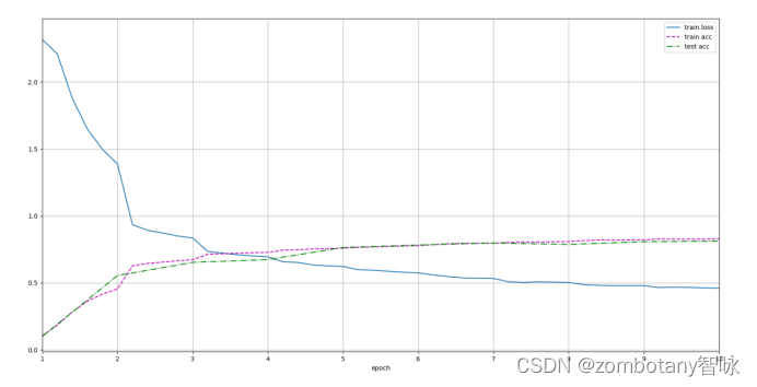
loss 0.460, train acc 0.829, test acc 0.812
5569.6 examples/sec on cpu

可以看到，正确地建立了经典的LeNet模型，在cpu上进行训练，最终结果为交叉熵函数loss为0.460。在训练集上准确率为0.829，测试集上准确率为0.812。在cpu上训练，每一秒只能运行5569.6个训练数据。
Epoch了10次，Loss函数、训练集准确率、测试集准确率变化曲线如下图所示。
在这里插入图片描述

六、总结及进一步改进设想

（主要总结本实验的不足以及进一步改进的设想）
总结：在本次实验中，使用了经典的基于CNN的LeNet算法，实现了对图片自动的特征提取与分类。深度学习的特点是存在一个甚至多个隐藏层(Hidden Layers)。
所以，深度学习比起传统机器学习方法的优点是：有隐藏层，能自动学习并完成特征提取任务，对于图像、自然语言、语音等非结构化的数据集，能够自动进行特征提取而不需要我们手动地构造相关特征，完成比一个简单的Sigmoid/Softmax函数更多的学习任务。比起简单的多层感知机、神经网络，卷积神经网络能够保留输入形状的特征，将统一卷积核与不同位置的输入重复计算，避免隐藏层权重参数尺寸过大。在结果上，测试的精度比起传统机器学习算法也有一定提升。
然而，深度学习方法也有缺点。深度学习需要消耗大量的内存、运算资源、时间进行训练。
本实验存在一定不足之处，需要进一步改进。由于在安装Pytorch与TensorFlow深度学习框架时，安装成了cpu版本的而不是gpu版本的，所以在笔记本电脑上只能epoch较少次数且每个epoch都需要很长的耗时。因此，需要安装gpu版本，以更高效地学习深度学习，完成深度学习实验。

【机器学习/人工智能】实验二：图像特征自动学习方法实践与分析

写在前面

一、实验目的与要求

二、实验内容

三、实验设备与环境

四、设计正文

4.1 分析与设计思路

4.2 主要算法源码

五、实验结果及分析

六、总结及进一步改进设想

猜你喜欢

【机器学习/人工智能】 实验二：图像特征自动学习方法实践与分析

写在前面

一、实验目的与要求

二、实验内容

三、实验设备与环境

四、设计正文

4.1 分析与设计思路

4.2 主要算法源码

五、实验结果及分析

六、总结及进一步改进设想

猜你喜欢

【机器学习/人工智能】实验二：图像特征自动学习方法实践与分析