【机器学习】 实验3：K均值聚类

介绍

在本实验中，将实现K均值聚类算法(K-means)并了解其在数据聚类上的工作原理及图像压缩上的应用。

本次实验需要用到的数据集包括：

• ex3data1.mat -2D 数据集
• hzau.jpeg -用于测试k均值聚类算法图像压缩性能的图像

评分标准如下：

• 要点1：寻找最近类中心点-----------------（20分）
• 要点2：计算均值类中心--------------------（20分）
• 要点3：随机初始化类中心-----------------（10分）
• 要点4：K均值聚类算法---------------------（20分）
• 要点5：图像压缩-----------------------------（30分）

# 引入所需要的库文件
import os
import numpy as np
import pandas as pd
import matplotlib.pyplot as plt
import matplotlib as mpl
import seaborn as sb
from scipy.io import loadmat

%matplotlib inline

1 K均值聚类 K-means Clustering

在本部分实验中，将实现K均值聚类算法。

在每次迭代中，算法主要包含两个部分：寻找最近类中心点和计算均值类中心。

另外，基于初始化的需求，需创建一个选择随机样本并将其用作初始聚类中心的函数。

1.1 寻找最近类中心点

在本部分实验中，我们将为每个样本点寻找离其距离最近的类中心，并将其赋予对应的类。

具体的更新公式如下：

 其中为第i个样本点，为第j个均值类中心。

**要点 1：** 在下方cell中，请**实现''寻找最近类中心点''的代码**。

# ====================== 在这里填入代码 =======================
def find_closest_centroids(X, centroids):
    """   
    输入
    ----------
    X : 尺寸为 (m, n)的矩阵，第i行为第i个样本，n为样本的维数。 
    centroids : 尺寸为 (k, n)的矩阵，其中k为类别个数。
    
    输出
    -------
    idx : 尺寸为 (m, 1)的矩阵，第i个分量表示第i个样本的类别。 
    """
    m = X.shape[0]
    k = centroids.shape[0]
    idx = np.zeros(m)
    
    for i in range(m):
        min_dist = 1e9
        for j in range(k):
            dist = np.sum((X[i,:] - centroids[j,:])** 2)
            if dist < min_dist:
                min_dist = dist
                idx[i] = j

    return idx
# ============================================================= 

如果完成了上述函数 find_closest_centroids，以下代码可用于测试。如果结果为[0 2 1]，则计算通过。

#导入数据
data = loadmat('ex3data1.mat')
X = data['X']
initial_centroids = np.array([[3, 3], [6, 2], [8, 5]])

idx = find_closest_centroids(X, initial_centroids)
idx[0:3]

输出结果：

#显示并查看部分数据
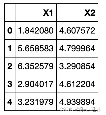
data2 = pd.DataFrame(data.get('X'), columns=['X1', 'X2'])
data2.head()

输出结果：

#可视化二维数据
fig, ax = plt.subplots(figsize=(9,6))
ax.scatter(X[:,0], X[:,1], s=30, color='k', label='Original')
ax.legend()
plt.show()

输出结果：

1.2 计算均值类中心

在本部分实验中，我们将每类样本的均值作为新的类中心。

具体的更新公式如下：

 其中为第j类样本点的指标集，∣∣∣∣为集合的元素个数。

**要点 2：** 在下方cell中，请**实现''计算均值类中心''的代码**。

# ====================== 在这里填入代码 ======================= 
def compute_centroids(X, idx, k):
    m, n = X.shape
    centroids = np.zeros((k,n))
    for i in range(k):
        indices =  np.where(idx == i)
        centroids[i,:] = (np.sum(X[indices,:], axis=1)/ len(indices[0])).ravel()
    return centroids
# ============================================================= 

#测试上述计算均值类中心代码
compute_centroids(X, idx, 3)

输出结果：

1.3 随机初始化类中心

随机选择k个样本作为初始类中心。

**要点 3：** 在下方cell中，请**实现''随机初始化类中心''的代码**。具体为随机选择k个样本作为初始类中心。

# ====================== 在这里填入代码 ======================= 
def init_centroids(X, k):
    m, n = X.shape
    idx = np.random.randint(0, m, k)
    centroids = np.zeros((k, n))
    for i in range(k):
        centroids[i,:] = X[idx[i],:]
    return centroids
# ============================================================= 

#测试上述随机初始化类中心代码
init_centroids(X, 3)

输出结果：

 1.4 实现K均值聚类算法

**要点 4：** 在下方cell中，请通过结合上述步骤**实现''K均值聚类算法''的代码**。

# ====================== 在这里填入代码 =======================
def run_k_means(X, initial_centroids, max_iters):
    m, n = X.shape
    k = initial_centroids.shape[0]
    idx = np.zeros(m)
    centroids = initial_centroids
    for i in range(max_iters):
        idx = find_closest_centroids(X, centroids)
        centroids = compute_centroids(X, idx, k)
        
    
    
    return idx, centroids
# ============================================================= 

2 将K均值聚类算法应用于数据集1

在本部分实验中，将已实现的K均值聚类算法应用于数据集1，该数据集中的样本维数为2，因此聚类结束后，可通过可视化观察聚类结果。

idx, centroids = run_k_means(X, initial_centroids, 10)

cluster1 = X[np.where(idx == 0)[0],:]
cluster2 = X[np.where(idx == 1)[0],:]
cluster3 = X[np.where(idx == 2)[0],:]

fig, ax = plt.subplots(figsize=(9,6))
ax.scatter(cluster1[:,0], cluster1[:,1], s=30, color='r', label='Cluster 1')
ax.scatter(cluster2[:,0], cluster2[:,1], s=30, color='g', label='Cluster 2')
ax.scatter(cluster3[:,0], cluster3[:,1], s=30, color='b', label='Cluster 3')
ax.legend()
plt.show()

输出结果：

 1.3 将K均值聚类算法应用于图像压缩 Image compression with K-means

#读取图像
A = mpl.image.imread('hzau.jpeg')
A.shape

输出结果：

现在我们需要对数据应用一些预处理，并将其提供给K-means算法。

# 归一化图像像素值的范围到[0, 1] 
A = A / 255.

# 对原始图像尺寸作变换
X = np.reshape(A, (A.shape[0] * A.shape[1], A.shape[2]))
X.shape

输出结果：

 **要点 5：** 在下方cell中，**请利用K均值聚类算法实现图像压缩**。具体方法是将原始像素替换为对应的均值类中心像素。

# ====================== 在这里填入代码 =======================
idx, centroids = run_k_means(X, initial_centroids, 10)
idx = find_closest_centroids(X, centroids)


A_compressed = centroids[idx.astype(int),:]
A_compressed.shape

print(A_compressed.shape)
# ============================================================= 

输出结果：

#显示压缩前后的图像
fig, ax = plt.subplots(1, 2, figsize=(9,6))
ax[0].imshow(A)
ax[0].set_axis_off()
ax[0].set_title('Original image')
ax[1].imshow(A_compressed)
ax[1].set_axis_off()
ax[1].set_title('Compressed image')
plt.show()

输出结果：