用Gurobi+python求解设施选址问题(facility location)

参考：Gurobi 官方资源

设施选址（Facility Location）

1.背景介绍

设施选址问题在许多工业领域如物流，通信等都有应用，在本案例中展示如何解决设施选址问题，决策出仓库的数量和地点，为一些超市供应。求解思路：问题建模成混合整数规划问题，用python调用Gurobi求解器实现。

设施选址问题也称为选址分析(location analysis)，是运筹优化领域的一个重要分支，要求选出设施的最佳位置，从而减小运输成本，同时考虑一些其它因素，如安全（避免在靠近居民地的地方存储有害物质）和竞争者的设施位置。

设施选址问题在很多领域都有应用，对于供应链和物流管理，这个问题可以用来找到商店，工厂和仓库的最佳位置，其它应用如公共策略（在城市中部署警局），通信（网络中的手机信号塔），甚至是粒子物理学（排斥电荷之间的间隔距离），天然气输送装备的选址等。最后，可以将设施点位置问题应用于聚类分析。

2.问题描述

一个大型的超市连锁店想要为它的一些超市修建仓库，超市的位置都已知，但是仓库的位置还没决定。
仓库选址有几个候选地，需要决定出修建几个仓库和确定这些仓库的位置。
修建仓库越多，就能减少卡车从仓库到超市的运输距离，因此减少运输成本，但是开设一个仓库有一个固定成本。
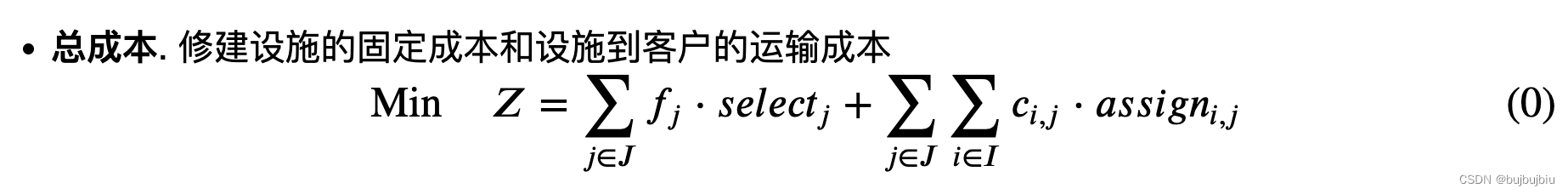
优化目标是最小化总成本=开始仓库固定成本+仓库到超市运输成本。

3.MIP模型

建立数学规划模型用gurobi求解，一个数学优化模型有5个部分：

• 集合和索引（Sets and indices）
• 参数（Parameters）
• 决策变量（Decision variables）
• 目标函数（Objective function(s)）
• 约束条件（Constraints）

接下来为设施选址问题构建MIP模型

（1）集合和索引

$i\in I$: 超市（顾客）位置的索引和集合.

$j\in J$: 候选仓库（设施）位置的索引和集合.

（2）参数

$f_j\in {\mathbb{R}}^{+}$: 修建设施 $j\in J$ 的固定成本.

$d_{i,j}\in {\mathbb{R}}^{+}$: 设施 $j\in J$ 和客户 $i\in I$ 的距离.

扫描二维码关注公众号，回复： 15188766 查看本文章

$c_{i,j}\in {\mathbb{R}}^{+}$: 候选设施地点 $j\in J$ 和客户点 $i\in I$ 的运输成本. 假设成本和距离成比例. 因此 $c_{i,j}=\alpha \cdot d_{i,j}$, $\alpha$ 是单位运输成本.

（3）决策变量

s e l e c t j ∈ { 0 , 1 } select_{j} \in \{0, 1 \} selectj​∈{ 0,1}: 如果在候选设施点 $j\in J$ 修建，值为1; 否则为0

$0\le assig{n}_{i,j}\le 1$: 非负连续变量，表明客户 $i\in I$ 从设施 $j\in J$ 接收需求的比例.

（4）目标函数

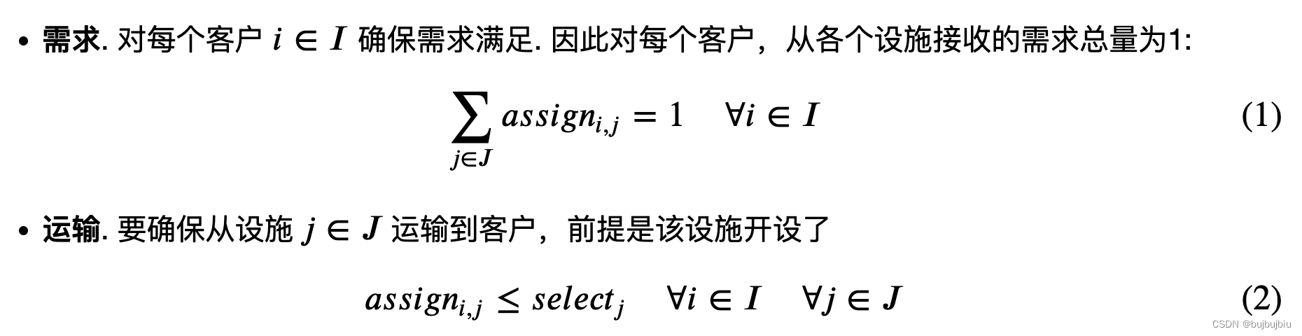
（5）约束条件

4.python调用gurobi实现

本例中考虑2个超市和9个候选仓库，每个超市的位置坐标如下

	Coordinates
Supermarket 1	(0,1.5)
Supermarket 2	(2.5,1.2)

下面的表格是候选仓库的坐标和修建固定成本，单位millions GBP

	coordinates	fixed cost
Warehouse 1	(0,0)	3
Warehouse 2	(0,1)	2
Warehouse 3	(0,2)	3
Warehouse 4	(1,0)	1
Warehouse 5	(1,1)	3
Warehouse 6	(1,2)	3
Warehouse 7	(2,0)	4
Warehouse 8	(2,1)	3
Warehouse 9	(2,2)	2

每mile的运输成本是1 million GBP

现在导入gurobi和其它python库，初始化给定数据的数据结构

from itertools import product
from math import sqrt

import gurobipy as gp
from gurobipy import GRB

customers = [(0,1.5), (2.5,1.2)]
facilities = [(0,0), (0,1), (0,2), (1,0), (1,1), (1,2), (2,0), (2,1), (2,2)]
setup_cost = [3,2,3,1,3,3,4,3,2]
cost_per_mile = 1

（1）预处理

定义一个函数，用于计算每个设施和客户之间的欧式距离，获取MIP模型需要的关键参数

# 计算两个地方的欧式距离
def compute_distance(loc1, loc2):
    dx = loc1[0] - loc2[0]
    dy = loc1[1] - loc2[1]
    return sqrt(dx*dx + dy*dy)

num_facilities = len(facilities)
num_customers = len(customers)
cartesian_prod = list(product(range(num_customers), range(num_facilities)))

# 每对客户和设施的运输成本
shipping_cost = {
    
    (c,f):cost_per_mile * compute_distance(customers[c], facilities[f]) 
                 for c,f in cartesian_prod}

shipping_cost

{(0, 0): 1.5,
 (0, 1): 0.5,
 (0, 2): 0.5,
 (0, 3): 1.8027756377319946,
 (0, 4): 1.118033988749895,
 (0, 5): 1.118033988749895,
 (0, 6): 2.5,
 (0, 7): 2.0615528128088303,
 (0, 8): 2.0615528128088303,
 (1, 0): 2.773084924772409,
 (1, 1): 2.5079872407968904,
 (1, 2): 2.6248809496813377,
 (1, 3): 1.9209372712298547,
 (1, 4): 1.5132745950421556,
 (1, 5): 1.7,
 (1, 6): 1.3,
 (1, 7): 0.5385164807134504,
 (1, 8): 0.9433981132056605}

（2）模型部署

现在定义设施选址问题的MIP模型，包括决策变量，约束和目标函数。然后开始优化过程，Gurobi找到能最小化总成本的修建方案

# 模型
m = gp.Model('facility_location')

# 两个决策变量
select = m.addVars(num_facilities, vtype=GRB.BINARY, name='select')
assign = m.addVars(cartesian_prod, ub=1, vtype=GRB.CONTINUOUS, name='assign')

# 两个约束条件
m.addConstrs((assign[c,f] <= select[f] for c,f in cartesian_prod), name='Setup2ship')
m.addConstrs((gp.quicksum(assign[c,f] for f in range(num_facilities)) == 1 for c in range(num_customers)),name='demand')

# 目标函数
m.setObjective(select.prod(setup_cost) + assign.prod(shipping_cost), GRB.MINIMIZE)

# 优化
m.optimize()

Set parameter Username
Academic license - for non-commercial use only - expires 2023-10-24
Gurobi Optimizer version 9.5.2 build v9.5.2rc0 (mac64[rosetta2])
Thread count: 8 physical cores, 8 logical processors, using up to 8 threads
Optimize a model with 20 rows, 27 columns and 54 nonzeros
Model fingerprint: 0x0939f503
Variable types: 18 continuous, 9 integer (9 binary)
Coefficient statistics:
  Matrix range     [1e+00, 1e+00]
  Objective range  [5e-01, 4e+00]
  Bounds range     [1e+00, 1e+00]
  RHS range        [1e+00, 1e+00]
Presolve time: 0.01s
Presolved: 20 rows, 27 columns, 54 nonzeros
Variable types: 18 continuous, 9 integer (9 binary)
Found heuristic solution: objective 6.0385165

Root relaxation: objective 4.723713e+00, 15 iterations, 0.00 seconds (0.00 work units)

    Nodes    |    Current Node    |     Objective Bounds      |     Work
 Expl Unexpl |  Obj  Depth IntInf | Incumbent    BestBd   Gap | It/Node Time

*    0     0               0       4.7237129    4.72371  0.00%     -    0s

Explored 1 nodes (15 simplex iterations) in 0.03 seconds (0.00 work units)
Thread count was 8 (of 8 available processors)

Solution count 2: 4.72371 6.03852 

Optimal solution found (tolerance 1.00e-04)
Best objective 4.723712908962e+00, best bound 4.723712908962e+00, gap 0.0000%

5.结果分析

优化模型结果显示最小成本是4.72 million GBP

（1）仓库修建计划

接下来看一下仓库修建选址决策：在位置4修建一个仓库

for facility in select.keys():
    if (abs(select[facility].x) > 1e-6):
        print(f"\n Build a warehouse at location {
      
      facility + 1}.")

 Build a warehouse at location 4.

（2）运输计划

运输计划表明了从每个修建的设施运送到每个客户的比例：两个超市都由仓库4供货

for customer, facility in assign.keys():
    if (abs(assign[customer, facility].x)) > 1e-6:
        print(f"\n Supermarket {
      
      customer + 1} receives {
      
      round(100*assign[customer, facility].x, 2)} % of its demand  from Warehouse {
      
      facility + 1} .")

 Supermarket 1 receives 100.0 % of its demand  from Warehouse 4 .

 Supermarket 2 receives 100.0 % of its demand  from Warehouse 4 .