目标和背景
采用逻辑回归方法,使用过去 5 天的收益率 X 来预测未来一天的涨跌 Y,
并依据涨跌概率大小来构建多空投资组合。
解决方案和程序
- 拟合模型:将其中 450 天数据作为训练样本,拟合一个逻辑回归模型,得
到参数估计。用最后 50 天数据作为预测样本,用于检验模型效果。 - 计算信息系数:检验样本中股票涨跌的预测和实际涨跌的相关系数大约为
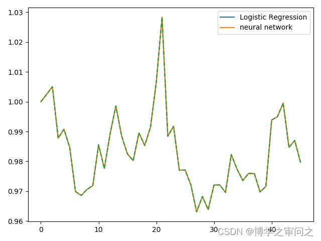
0.077,即信息系数,用来度量因子或因子组合的好坏。 - 构建多空投资组合:等比例持有预测上涨概率最大的 10 支股票,做空上
涨概率最小的 10 支股票,画出组合收益图。
参考代码:
import numpy as np
import numpy.linalg as la
import pandas as pd
import os
import matplotlib.pyplot as plt
index_path = r’data\SZ399300.TXT’
index300 = pd.read_table(index_path,
encoding = ‘cp936’,header = None)
idx = index300[:-1]
idx.columns = [‘date’,‘o’,‘h’,‘l’,‘c’,‘v’,‘to’]
idx.index = idx[‘date’]
stock_path = r’data\hs300’
names = os.listdir(stock_path)
close = []
for name in names:
spath = stock_path + ‘\’ + name
df0 = pd.read_table(spath,
encoding = ‘cp936’,header = None)
df1 = df0[:-1]
df1.columns = [‘date’,‘o’,‘h’,‘l’,‘c’,‘v’,‘to’]
df1.index = df1[‘date’]
df2 = df1.reindex(idx.index,method = ‘ffill’)
df3 = df2.fillna(method = ‘bfill’)
close.append(df3[‘c’].values)
data = np.asarray(close).T
retx = (data[1:,:]-data[:-1,:])/data[:-1,:]
n = 500
n1 = 50
p = 5
train = retx[-n:-n1,:]
ret = train[p:,:].ravel()
X1 = train[4:-1,:].ravel()[:,np.newaxis]
X2 = train[3:-2,:].ravel()[:,np.newaxis]
X3 = train[2:-3,:].ravel()[:,np.newaxis]
X4 = train[1:-4,:].ravel()[:,np.newaxis]
X5 = train[:-5,:].ravel()[:,np.newaxis]
y_train = (ret>0).astype(int)
X_train = np.hstack((X5,X4,X3,X2,X1))
test = retx[-n1:,:]
ret2 = test[p:,:].ravel()
X1 = test[4:-1,:].ravel()[:,np.newaxis]
X2 = test[3:-2,:].ravel()[:,np.newaxis]
X3 = test[2:-3,:].ravel()[:,np.newaxis]
X4 = test[1:-4,:].ravel()[:,np.newaxis]
X5 = test[:-5,:].ravel()[:,np.newaxis]
y_test = (ret2>0).astype(int)
X_test = np.hstack((X5,X4,X3,X2,X1))
from sklearn import linear_model
from sklearn.metrics import classification_report
clf = linear_model.LogisticRegression(C=1e2,fit_intercept=True)
clf.fit(X_train,y_train)
y_pred0 = clf.predict(X_train)
print(classification_report(y_train, y_pred0))
np.corrcoef([y_train,y_pred0])
y_pred = clf.predict(X_test)
from sklearn.metrics import classification_report
print(classification_report(y_test, y_pred))
np.corrcoef([y_test,y_pred]) # Information Coefficient, IC
holding_matrix = np.zeros((n1-p,300))
for j in range(n1-p):
#prob = clf.predict_proba(test[j:j+5,:].T)[:,1]
prob = clf.predict_proba(test[j:j+p,:].T)[:,1]
long_position = prob.argsort()[-10:]
short_position = prob.argsort()[:10]
holding_matrix[j,long_position] = 0.05
holding_matrix[j,short_position] = -0.05
tmp_ret = np.sum(holding_matrix*test[p:],axis = 1)
portfolio_ret = np.append(0,tmp_ret)
plt.plot(np.cumprod(1+portfolio_ret))
plt.legend([‘Performance of LR’],loc=‘upper left’)
plt.savefig(r’fig\stockret-lr’)
plt.plot(np.cumprod(1+portfolio_ret))
plt.plot(np.cumprod(1+portfolio_ret),‘–’)
plt.legend([‘Logistic Regression’,‘neural network’])
plt.savefig(r’fig\stockret-lrnn’)
plt.show()
运行结果: