第一次通过Tensorflow对象检测API了解对象检测。它很容易使用。传入了一张海滩的图片,作为回报,API在它识别的对象上绘制了方框。这似乎很神奇。
很好奇,想剖析API,了解它到底是如何在幕后工作的。这很难,我失败了。Tensorflow对象检测API支持经过数十年研究的最先进模型。它们被复杂地编织成代码,就像钟表匠如何将微小的齿轮组合在一起,它们可以连贯地移动。
然而,目前大多数最先进的模型都建立在Faster RCNN模型的基础之上,即使在今天,该模型仍然是计算机视觉领域被引用最多的论文之一。因此,理解它至关重要。
在本文中,我们将分解Faster RCNN论文,了解其工作原理,并在PyTorch中部分构建它,以了解其中的细微差别。
Faster R-CNN概述
对于物体检测,我们需要建立一个模型,并教它学会识别和定位图像中的物体。
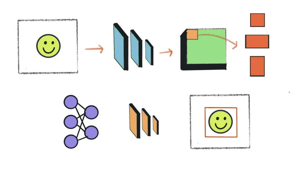
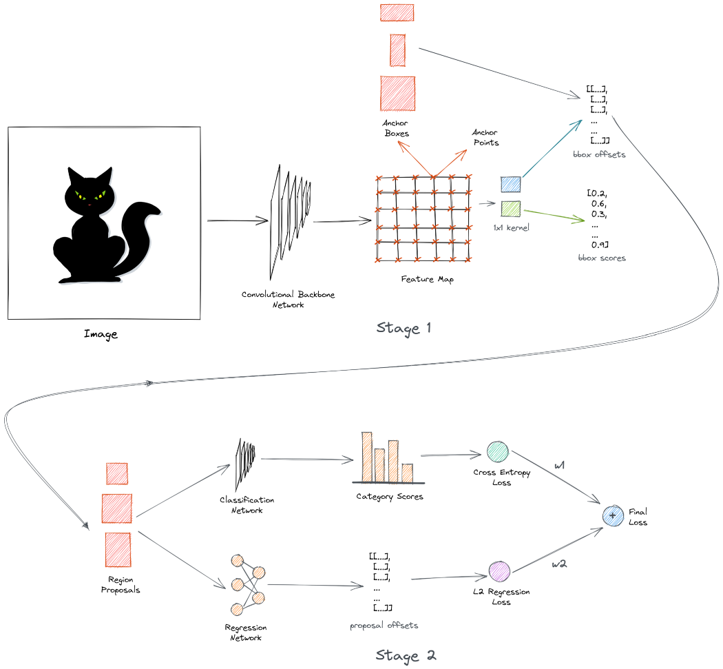
Faster R-CNN模型采用以下方法:图像首先通过主干网络获得输出特征图,主干网络通常是卷积网络,如ResNet或VGG16。输出特征图是表示图像的学习特征的空间密集张量。接下来,我们生成多个不同大小和形状的框。这些定位框的目的是捕获图像中的对象。
我们使用1x1卷积网络来预测所有锚盒的类别和偏移。在训练期间,我们对与标签重叠最多的锚框进行采样。这些被称为阳性或正锚框。我们还对与标签锚框几乎没有重叠的负锚框进行了采样。
网络学习使用二进制交叉熵损失对锚盒进行分类。现在,正锚框可能与标签锚框不完全对齐。因此,我们训练了一个类似的1x1卷积网络,以学习从标签锚框预测偏移。当应用于锚框时,这些偏移会使它们更接近标签锚框。
我们使用L2回归损失来学习偏移。使用预测的偏移来变换锚框,并将其称为区域建议,并且上述网络称为区域提议网络。这是探测器的第一阶段。Faster RCNN是一个两级检测器。还有另一个阶段。
第2阶段的输入是从第1阶段生成的区域建议。在第2阶段,我们学习使用简单的卷积网络预测区域建议中的对象类别。现在,建议的框大小不同,因此我们使用一种称为ROI池的技术在通过网络之前调整它们的大小。该网络学习使用交叉熵损失来预测多个类别。
我们使用另一个网络来预测来自标签锚框的区域提议的偏移量。这一网络进一步试图使预测的框与标签锚框保持一致。这使用L2回归损失。最后,我们对两种损失进行加权组合,以计算最终损失。在第二阶段,我们学习预测类别和偏移量。这被称为多任务学习。
所有这些都发生在训练期间。在推断过程中,我们通过主干网络传递图像并生成锚框-与之前相同。然而,这一次我们只选择在第一阶段中获得高分类分数的前300个框,并使它们有资格进入第二阶段。
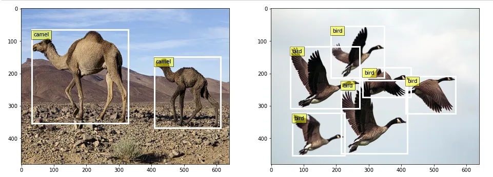
在第二阶段,我们预测最终类别和偏移量。此外,我们还执行了一个额外的后处理步骤,使用一种称为非最大抑制的技术来删除重复的边界框。如果一切按预期运行,探测器会识别并在图像中的对象上绘制方框,如下所示:
这是两阶段Faster RCNN网络的简要概述。在接下来的部分中,我们将深入探讨每个部分。
设置环境
使用的所有代码都可以在此GitHub存储库中找到。我们不需要很多依赖项,因为我们将从头开始构建。仅在标准anaconda环境中安装PyTorch库就足够了。
https://github.com/wingedrasengan927/pytorch-tutorials/tree/master/Object%20Detection
这是我们要使用的主要笔记本
https://gist.github.com/wingedrasengan927/3d5eb6f1b0d4fb3acbf2550f9db8daf0#file-faster-r-cnn-ipynb
%load_ext autoreload
%autoreload 2
import numpy as np
from skimage import io
from skimage.transform import resize
import matplotlib.pyplot as plt
import random
import matplotlib.patches as patches
from utils import *
from model import *
import os
import torch
import torchvision
from torchvision import ops
import torch.nn as nn
import torch.nn.functional as F
from torch.utils.data import DataLoader, Dataset
from torch.nn.utils.rnn import pad_sequence准备和加载数据
首先,我们需要使用一些示例图像。这里我从这里下载了两张高分辨率图像。
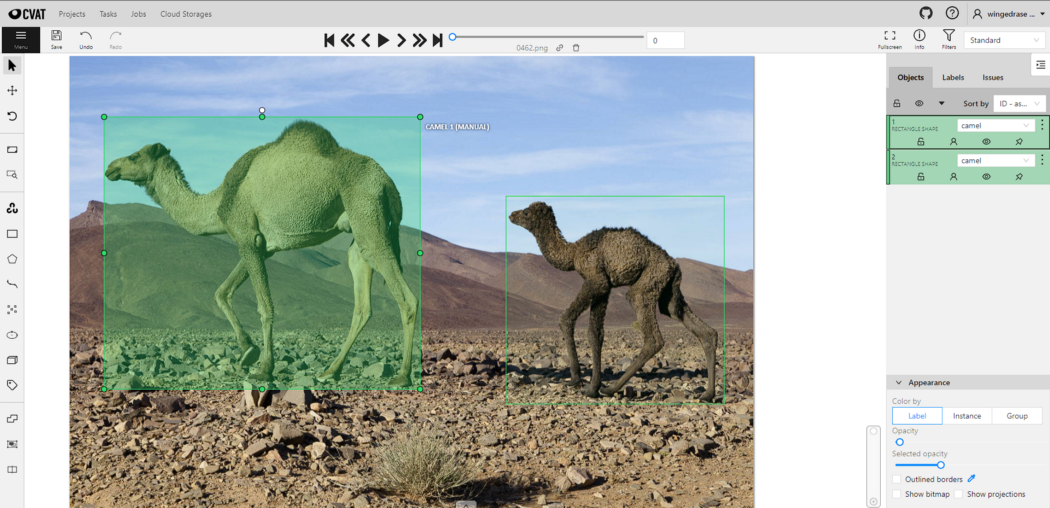
接下来,我们需要标记这些图像。CVAT是目前流行的开源标签工具之一。
你只需将图像加载到工具中,在相关对象周围绘制框,并标记其类别,如下所示:
完成后,可以将注释导出为首选格式。在这里,我已经将它们导出为CVAT for images 1.1 xml格式。
注释文件包含有关图像、标记类和边界框坐标的所有信息。
PyTorch数据集和DataLoader
在PyTorch中,创建一个继承自PyTorch的Dataset类的类来加载数据被认为是最佳实践。这将使我们对数据有更多的控制,并有助于保持代码模块化。此外,我们可以从数据集实例创建PyTorch DataLoader,它可以自动处理数据的批处理、混洗和采样。
class ObjectDetectionDataset(Dataset):
    '''
    A Pytorch Dataset class to load the images and their corresponding annotations.

    Returns
    ------------
    images: torch.Tensor of size (B, C, H, W)
    gt bboxes: torch.Tensor of size (B, max_objects, 4)
    gt classes: torch.Tensor of size (B, max_objects)
    '''
    def __init__(self, annotation_path, img_dir, img_size, name2idx):
        self.annotation_path = annotation_path
        self.img_dir = img_dir
        self.img_size = img_size
        self.name2idx = name2idx

        self.img_data_all, self.gt_bboxes_all, self.gt_classes_all = self.get_data()

    def __len__(self):
        return self.img_data_all.size(dim=0)

    def __getitem__(self, idx):
        return self.img_data_all[idx], self.gt_bboxes_all[idx], self.gt_classes_all[idx]

    def get_data(self):
        img_data_all = []
        gt_idxs_all = []

        gt_boxes_all, gt_classes_all, img_paths = parse_annotation(self.annotation_path, self.img_dir, self.img_size)

        for i, img_path in enumerate(img_paths):

            # skip if the image path is not valid
            if (not img_path) or (not os.path.exists(img_path)):
                continue

            # read and resize image
            img = io.imread(img_path)
            img = resize(img, self.img_size)

            # convert image to torch tensor and reshape it so channels come first
            img_tensor = torch.from_numpy(img).permute(2, 0, 1)

            # encode class names as integers
            gt_classes = gt_classes_all[i]
            gt_idx = torch.Tensor([self.name2idx[name] for name in gt_classes])

            img_data_all.append(img_tensor)
            gt_idxs_all.append(gt_idx)

        # pad bounding boxes and classes so they are of the same size
        gt_bboxes_pad = pad_sequence(gt_boxes_all, batch_first=True, padding_value=-1)
        gt_classes_pad = pad_sequence(gt_idxs_all, batch_first=True, padding_value=-1)

        # stack all images
        img_data_stacked = torch.stack(img_data_all, dim=0)

        return img_data_stacked.to(dtype=torch.float32), gt_bboxes_pad, gt_classes_pad
在上面的类中,我们定义了一个名为get_data的函数,该函数加载注释文件并解析它以提取图像路径、标记类和边界框坐标,然后将其转换为PyTorch的Tensor对象。图像将被重塑为固定大小。
注意,我们正在填充边界框。这与调整大小相结合,允许我们将图像批处理在一起。

我们可以从DataLoader中获取一些图像并将其可视化,如下所示:

主干网络
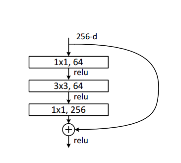
这里我们将使用ResNet 50作为主干网络。记住,ResNet 50中的单个块由瓶颈层的堆栈组成。在沿空间维度的每个块之后,图像会减少一半,而通道的数量会增加一倍。瓶颈层由三个卷积层以及跳跃连接组成,如下所示:
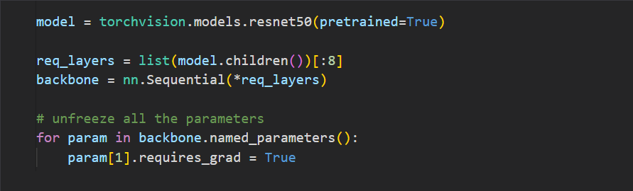
我们将使用ResNet 50的前四个块作为主干网络。
一旦图像通过主干网络,它就会沿着空间维度向下采样。输出是图像的特征丰富的表示。
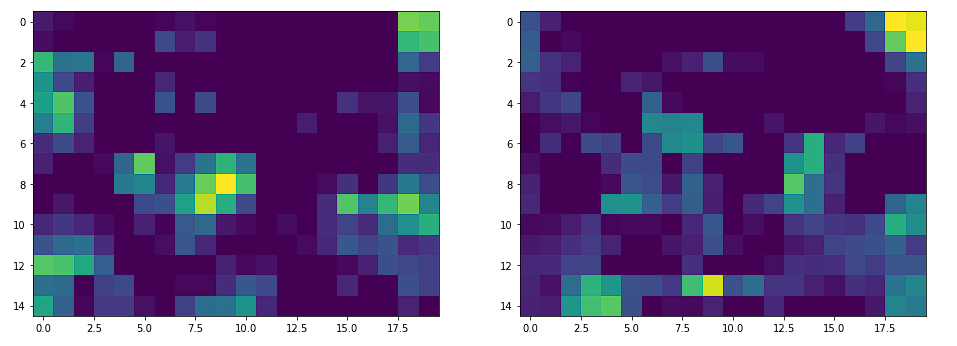
如果我们通过主干网络传递大小(640、480)的图像,我们将得到大小(15、20)的输出特征图。因此,图像已缩小(32,32)。
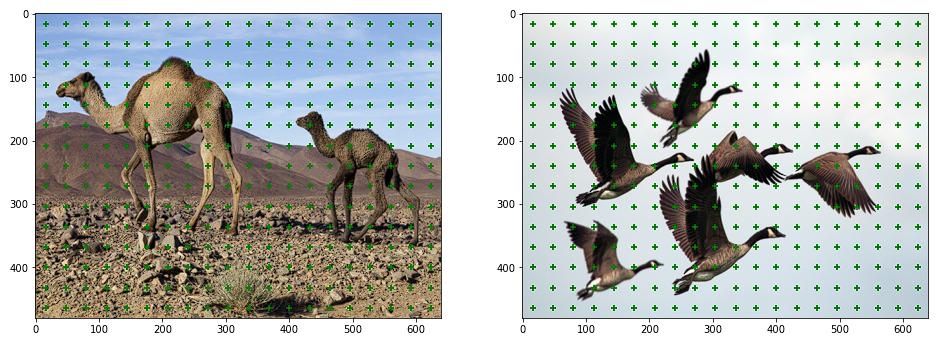
生成锚点
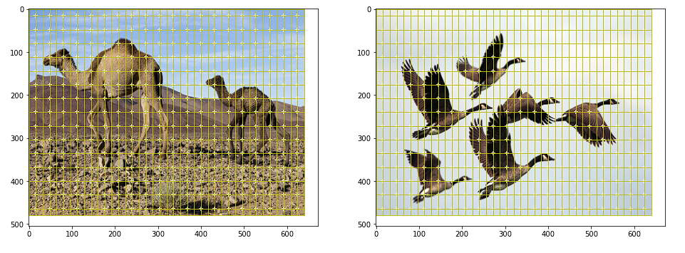
我们将特征图中的每个点视为锚点。因此,锚点将只是表示沿宽度和高度维度的坐标的数组。
def gen_anc_centers(out_size):
    out_h, out_w = out_size

    anc_pts_x = torch.arange(0, out_w) + 0.5
    anc_pts_y = torch.arange(0, out_h) + 0.5

    return anc_pts_x, anc_pts_y
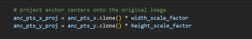
为了可视化这些锚点,我们可以简单地通过乘以宽度和高度比例因子将它们投影到图像空间上。
生成锚框
对于每个锚点,我们生成九个不同形状和大小的边界框。我们选择这些框的大小和形状,以便它们包围图像中的所有对象。锚框的选择通常取决于数据集。
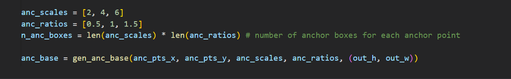
def gen_anc_base(anc_pts_x, anc_pts_y, anc_scales, anc_ratios, out_size):
n_anc_boxes = len(anc_scales) * len(anc_ratios)
anc_base = torch.zeros(1, anc_pts_x.size(dim=0) \
, anc_pts_y.size(dim=0), n_anc_boxes, 4) # shape - [1, Hmap, Wmap, n_anchor_boxes, 4]
for ix, xc in enumerate(anc_pts_x):
for jx, yc in enumerate(anc_pts_y):
anc_boxes = torch.zeros((n_anc_boxes, 4))
c = 0
for i, scale in enumerate(anc_scales):
for j, ratio in enumerate(anc_ratios):
w = scale * ratio
h = scale
xmin = xc - w / 2
ymin = yc - h / 2
xmax = xc + w / 2
ymax = yc + h / 2
anc_boxes[c, :] = torch.Tensor([xmin, ymin, xmax, ymax])
c += 1
anc_base[:, ix, jx, :] = ops.clip_boxes_to_image(anc_boxes, size=out_size)
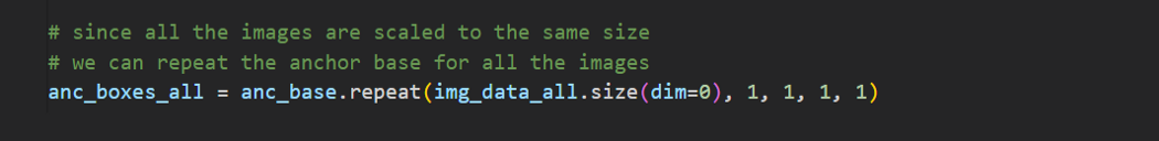
return anc_base调整图像大小的另一个优点是可以在所有图像上复制锚框。
再次,为了可视化锚框,我们通过乘以宽度和高度比例因子将其投影到图像空间。
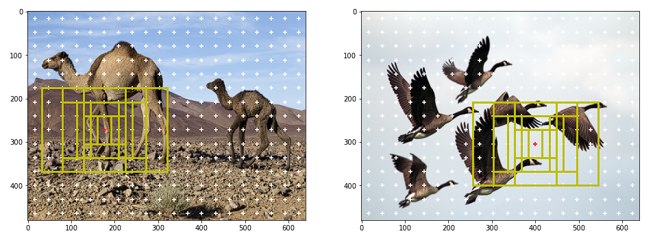
如果我们将所有锚点的所有锚框可视化,会出现以下情况:
数据准备
在本节中,我们将讨论训练的数据准备。
正负锚箱
我们只需要抽样几个锚盒进行训练。我们对正和负锚框进行采样。
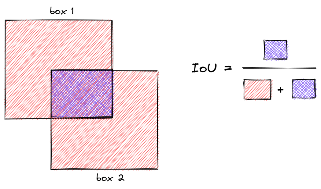
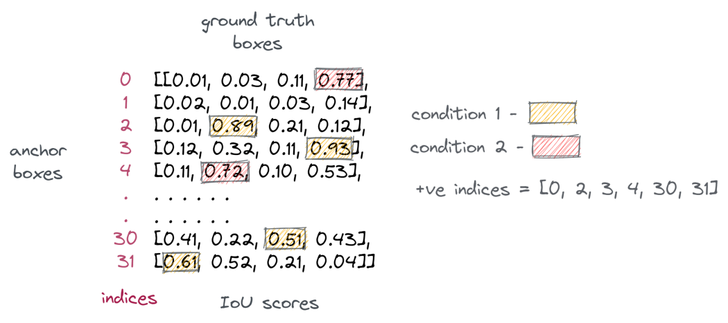
正框包含对象,负框不包含对象。为了对正锚框进行采样,我们选择IoU大于0.7的锚框和任何标签锚框。当锚框生成不好时,条件1失败,因此条件2会出现问题,因为它为每个标签锚框选择一个正框。为了对负锚框进行采样,我们选择IoU小于0.3的锚框。通常,阴性样本的数量将远远高于阳性样本。所以我们随机抽取一些样本,以匹配阳性样本的数量。IoU是度量两个边界框之间重叠的度量。
def get_iou_mat(batch_size, anc_boxes_all, gt_bboxes_all):
# flatten anchor boxes
anc_boxes_flat = anc_boxes_all.reshape(batch_size, -1, 4)
# get total anchor boxes for a single image
tot_anc_boxes = anc_boxes_flat.size(dim=1)
# create a placeholder to compute IoUs amongst the boxes
ious_mat = torch.zeros((batch_size, tot_anc_boxes, gt_bboxes_all.size(dim=1)))
# compute IoU of the anc boxes with the gt boxes for all the images
for i in range(batch_size):
gt_bboxes = gt_bboxes_all[i]
anc_boxes = anc_boxes_flat[i]
ious_mat[i, :] = ops.box_iou(anc_boxes, gt_bboxes)
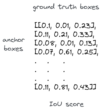
return ious_mat上面的函数计算IoU矩阵,其中包含图像中所有标签锚框的每个锚框的IoU。它将形状为(B,w_amap,h_amap,n_anc_boxes,4)的锚框和形状为(a,max_objects,4))的标签锚框作为输入,并返回一个形状矩阵(B,anc_boxes_tot,max_oobjects),其中符号如下:
B - Batch Size
w_amap - width of the output activation map
h_wmap - height of the output activation map
n_anc_boxes - number of anchor boxes per an anchor point
max_objects - max number of objects in a batch of images
anc_boxes_tot - total number of anchor boxes in the image i.e, w_amap * h_amap * n_anc_boxes
该函数基本上使所有锚框变平,并使用每个标签锚框计算IoU,如下所示:
投影标签锚框
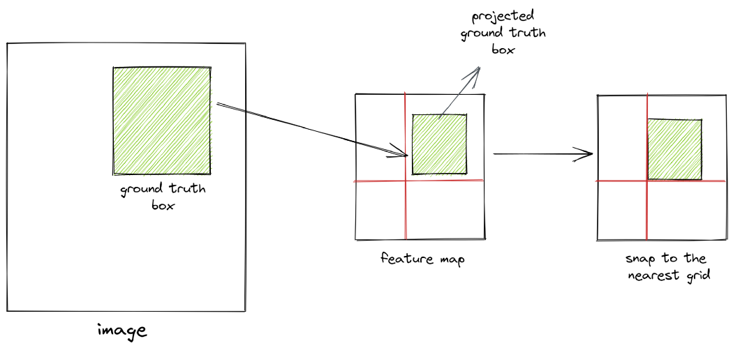
重要的是要记住,IoU是在生成的锚框和投影的标签锚框之间的特征空间中计算的。要将标签锚框投影到特征空间,我们只需将其坐标除以比例因子,如下函数所示:
def project_bboxes(bboxes, width_scale_factor, height_scale_factor, mode='a2p'):
    assert mode in ['a2p', 'p2a']

    batch_size = bboxes.size(dim=0)
    proj_bboxes = bboxes.clone().reshape(batch_size, -1, 4)
    invalid_bbox_mask = (proj_bboxes == -1) # indicating padded bboxes

    if mode == 'a2p':
        # activation map to pixel image
        proj_bboxes[:, :, [0, 2]] *= width_scale_factor
        proj_bboxes[:, :, [1, 3]] *= height_scale_factor
    else:
        # pixel image to activation map
        proj_bboxes[:, :, [0, 2]] /= width_scale_factor
        proj_bboxes[:, :, [1, 3]] /= height_scale_factor

    proj_bboxes.masked_fill_(invalid_bbox_mask, -1) # fill padded bboxes back with -1
    proj_bboxes.resize_as_(bboxes)

    return proj_bboxes
现在,当我们将坐标除以比例因子时,我们将值舍入为最接近的整数。这本质上意味着我们正在将标签锚框“捕捉”到特征空间中最近的网格。因此,如果图像空间和特征空间的尺度差异很大,我们将无法获得准确的投影。因此,在目标检测中使用高分辨率图像非常重要。
计算偏移量
正锚框与标签锚框不完全对齐。因此,我们计算正锚框和标签锚框之间的偏移,并训练神经网络来学习这些偏移。偏移量的计算方法如下:
tx_ = (gt_cx - anc_cx) / anc_w
ty_ = (gt_cy - anc_cy) / anc_h
tw_ = log(gt_w / anc_w)
th_ = log(gt_h / anc_h)

Where:

gt_cx, gt_cy - centers of ground truth boxes
anc_cx, anc_cy - centers of anchor boxes
gt_w, gt_h - width and height of ground truth boxes
anc_w, anc_h - width and height of anchor boxes
以下函数可用于计算相同值:
def calc_gt_offsets(pos_anc_coords, gt_bbox_mapping):
    pos_anc_coords = ops.box_convert(pos_anc_coords, in_fmt='xyxy', out_fmt='cxcywh')
    gt_bbox_mapping = ops.box_convert(gt_bbox_mapping, in_fmt='xyxy', out_fmt='cxcywh')

    gt_cx, gt_cy, gt_w, gt_h = gt_bbox_mapping[:, 0], gt_bbox_mapping[:, 1], gt_bbox_mapping[:, 2], gt_bbox_mapping[:, 3]
    anc_cx, anc_cy, anc_w, anc_h = pos_anc_coords[:, 0], pos_anc_coords[:, 1], pos_anc_coords[:, 2], pos_anc_coords[:, 3]

    tx_ = (gt_cx - anc_cx)/anc_w
    ty_ = (gt_cy - anc_cy)/anc_h
    tw_ = torch.log(gt_w / anc_w)
    th_ = torch.log(gt_h / anc_h)

    return torch.stack([tx_, ty_, tw_, th_], dim=-1)
如果你注意到,我们正在教网络了解锚框与标签锚框的距离。我们没有强迫它预测锚盒的确切位置和规模。因此,网络学习的偏移和变换是位置和尺度不变的。
代码演练
让我们浏览一下数据准备代码。这可能是整个存储库中最重要的函数。
def get_req_anchors(anc_boxes_all, gt_bboxes_all, gt_classes_all, pos_thresh=0.7, neg_thresh=0.2):
    '''
    Prepare necessary data required for training

    Input
    ------
    anc_boxes_all - torch.Tensor of shape (B, w_amap, h_amap, n_anchor_boxes, 4)
        all anchor boxes for a batch of images
    gt_bboxes_all - torch.Tensor of shape (B, max_objects, 4)
        padded ground truth boxes for a batch of images
    gt_classes_all - torch.Tensor of shape (B, max_objects)
        padded ground truth classes for a batch of images

    Returns
    ---------
    positive_anc_ind -  torch.Tensor of shape (n_pos,)
        flattened positive indices for all the images in the batch
    negative_anc_ind - torch.Tensor of shape (n_pos,)
        flattened positive indices for all the images in the batch
    GT_conf_scores - torch.Tensor of shape (n_pos,), IoU scores of +ve anchors
    GT_offsets -  torch.Tensor of shape (n_pos, 4),
        offsets between +ve anchors and their corresponding ground truth boxes
    GT_class_pos - torch.Tensor of shape (n_pos,)
        mapped classes of +ve anchors
    positive_anc_coords - (n_pos, 4) coords of +ve anchors (for visualization)
    negative_anc_coords - (n_pos, 4) coords of -ve anchors (for visualization)
    positive_anc_ind_sep - list of indices to keep track of +ve anchors
    '''
    # get the size and shape parameters
    B, w_amap, h_amap, A, _ = anc_boxes_all.shape
    N = gt_bboxes_all.shape[1] # max number of groundtruth bboxes in a batch

    # get total number of anchor boxes in a single image
    tot_anc_boxes = A * w_amap * h_amap

    # get the iou matrix which contains iou of every anchor box
    # against all the groundtruth bboxes in an image
    iou_mat = get_iou_mat(B, anc_boxes_all, gt_bboxes_all)

    # for every groundtruth bbox in an image, find the iou
    # with the anchor box which it overlaps the most
    max_iou_per_gt_box, _ = iou_mat.max(dim=1, keepdim=True)

    # get positive anchor boxes

    # condition 1: the anchor box with the max iou for every gt bbox
    positive_anc_mask = torch.logical_and(iou_mat == max_iou_per_gt_box, max_iou_per_gt_box > 0)

    # condition 2: anchor boxes with iou above a threshold with any of the gt bboxes
    positive_anc_mask = torch.logical_or(positive_anc_mask, iou_mat > pos_thresh)

    positive_anc_ind_sep = torch.where(positive_anc_mask)[0] # get separate indices in the batch
    # combine all the batches and get the idxs of the +ve anchor boxes
    positive_anc_mask = positive_anc_mask.flatten(start_dim=0, end_dim=1)
    positive_anc_ind = torch.where(positive_anc_mask)[0]

    # for every anchor box, get the iou and the idx of the
    # gt bbox it overlaps with the most
    max_iou_per_anc, max_iou_per_anc_ind = iou_mat.max(dim=-1)
    max_iou_per_anc = max_iou_per_anc.flatten(start_dim=0, end_dim=1)

    # get iou scores of the +ve anchor boxes
    GT_conf_scores = max_iou_per_anc[positive_anc_ind]

    # get gt classes of the +ve anchor boxes

    # expand gt classes to map against every anchor box
    gt_classes_expand = gt_classes_all.view(B, 1, N).expand(B, tot_anc_boxes, N)

    # for every anchor box, consider only the class of the gt bbox it overlaps with the most
    GT_class = torch.gather(gt_classes_expand, -1, max_iou_per_anc_ind.unsqueeze(-1)).squeeze(-1)

    # combine all the batches and get the mapped classes of the +ve anchor boxes
    GT_class = GT_class.flatten(start_dim=0, end_dim=1)
    GT_class_pos = GT_class[positive_anc_ind]

    # get gt bbox coordinates of the +ve anchor boxes

    # expand all the gt bboxes to map against every anchor box
    gt_bboxes_expand = gt_bboxes_all.view(B, 1, N, 4).expand(B, tot_anc_boxes, N, 4)
    # for every anchor box, consider only the coordinates of the gt bbox it overlaps with the most
    GT_bboxes = torch.gather(gt_bboxes_expand, -2, max_iou_per_anc_ind.reshape(B, tot_anc_boxes, 1, 1).repeat(1, 1, 1, 4))
    # combine all the batches and get the mapped gt bbox coordinates of the +ve anchor boxes
    GT_bboxes = GT_bboxes.flatten(start_dim=0, end_dim=2)
    GT_bboxes_pos = GT_bboxes[positive_anc_ind]

    # get coordinates of +ve anc boxes
    anc_boxes_flat = anc_boxes_all.flatten(start_dim=0, end_dim=-2) # flatten all the anchor boxes
    positive_anc_coords = anc_boxes_flat[positive_anc_ind]

    # calculate gt offsets
    GT_offsets = calc_gt_offsets(positive_anc_coords, GT_bboxes_pos)

    # get -ve anchors

    # condition: select the anchor boxes with max iou less than the threshold
    negative_anc_mask = (max_iou_per_anc < neg_thresh)
    negative_anc_ind = torch.where(negative_anc_mask)[0]
    # sample -ve samples to match the +ve samples
    negative_anc_ind = negative_anc_ind[torch.randint(0, negative_anc_ind.shape[0], (positive_anc_ind.shape[0],))]
    negative_anc_coords = anc_boxes_flat[negative_anc_ind]

    return positive_anc_ind, negative_anc_ind, GT_conf_scores, GT_offsets, GT_class_pos, \
         positive_anc_coords, negative_anc_coords, positive_anc_ind_sep
首先,我们使用上述函数计算IoU矩阵。然后从这个矩阵中,我们得到每个标签锚框的最重叠锚框的IoU。这是对正极锚盒进行采样的条件1。我们还应用条件2并选择IoU大于图像中任何标签锚框阈值的锚框。我们将条件1和条件2与所有图像的正锚框样本相结合。
每个图像将具有不同数量的阳性样本。为了避免训练过程中的这种差异,我们将批次压平并组合所有图像中的阳性样本。此外,我们可以使用torch.where跟踪每个阳性样本的来源。
接下来,我们需要计算来自标签样本的偏移量。为此,我们需要将每个阳性样本映射到其对应的标签锚框。需要注意的是,一个正锚框只能映射到一个标签锚框,而多个正锚盒可以映射到同一个标签锚框。
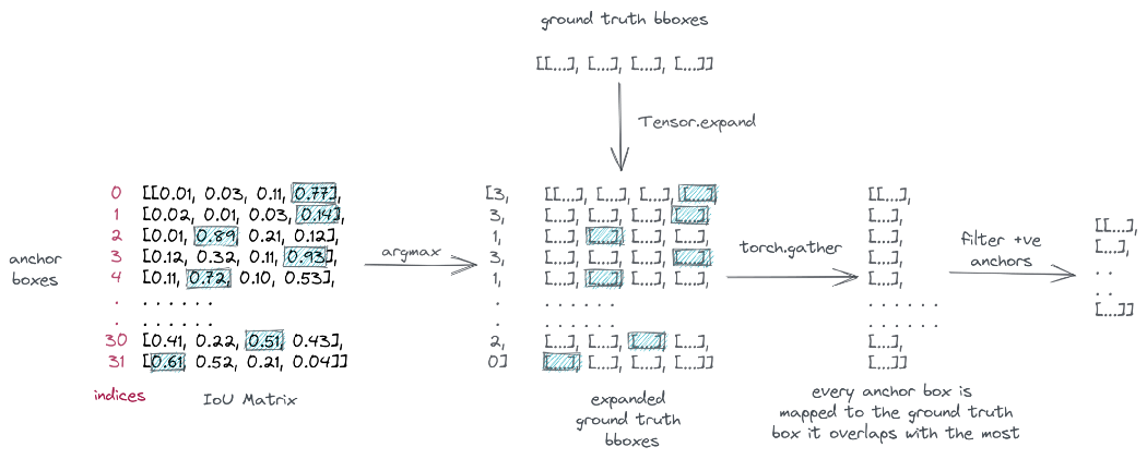
为了进行映射,我们首先使用Tensor.expand扩展标签锚框以匹配总的锚框。然后,对于每个锚框,我们选择其重叠最多的标签锚框。
为此,我们从IoU矩阵中获取所有锚框的最大IoU索引,然后使用torch.collect对这些索引进行“聚集”。最后,我们将批次压平并过滤阳性样本。该过程如下所示:
将每个锚框映射到其重叠最多的标签锚框
我们对类别执行相同的过程,为每个阳性样本分配一个类别。
现在我们已经为每个阳性样本映射了标签锚框,我们可以使用上述函数计算偏移量。
最后,我们通过使用所有标签锚框对IoU小于给定阈值的锚框进行采样来选择阴性样本。由于阴性样本的数量远远超过阳性样本,我们随机选择其中的一些样本来匹配计数。
下面是正负锚框的外观:
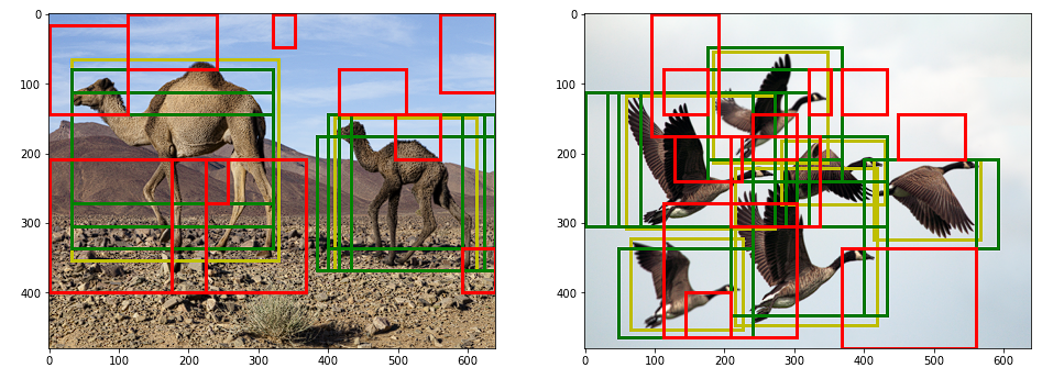
我们现在可以使用采样的正负锚框进行训练。
建立模型
建议模块
让我们先从建议模块开始。正如我们所讨论的,特征图中的每个点都被视为锚点,每个锚点都会生成不同大小和形状的框。我们希望将这些框中的每一个分类为对象或背景。
此外,我们希望从相应的标签锚框中预测它们的偏移量。我们怎么能做到这一点?解决方案是使用1x1卷积层。现在,1x1卷积层不会增加感受野。它们的功能不是学习图像级特征。它们相当于用来改变过滤器的数量,或者用作回归或分类头。
因此,我们采用两个1x1卷积层,并使用其中一个将每个锚框分类为对象或背景。我们称之为信心头。因此,给定大小为(B,C,w_amap,h_amap)的特征图,我们用卷积大小为1x1的核以获得大小为(B,n_anc_boxes,w_amap,h_amp)的输出。本质上,每个输出表示锚框的分类分数。
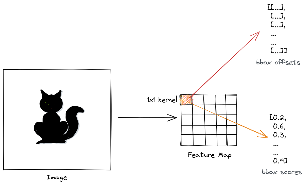
以类似的方式,另一个1x1卷积层获取特征图并产生大小(B,n_anc_boxes*4,w_amap,h_amap)的输出,其中输出滤波器表示锚框的预测偏移。这被称为回归头。
class ProposalModule(nn.Module):
    def __init__(self, in_features, hidden_dim=512, n_anchors=9, p_dropout=0.3):
        super().__init__()
        self.n_anchors = n_anchors
        self.conv1 = nn.Conv2d(in_features, hidden_dim, kernel_size=3, padding=1)
        self.dropout = nn.Dropout(p_dropout)
        self.conf_head = nn.Conv2d(hidden_dim, n_anchors, kernel_size=1)
        self.reg_head = nn.Conv2d(hidden_dim, n_anchors * 4, kernel_size=1)

    def forward(self, feature_map, pos_anc_ind=None, neg_anc_ind=None, pos_anc_coords=None):
        # determine mode
        if pos_anc_ind is None or neg_anc_ind is None or pos_anc_coords is None:
            mode = 'eval'
        else:
            mode = 'train'

        out = self.conv1(feature_map)
        out = F.relu(self.dropout(out))

        reg_offsets_pred = self.reg_head(out) # (B, A*4, hmap, wmap)
        conf_scores_pred = self.conf_head(out) # (B, A, hmap, wmap)

        if mode == 'train':
            # get conf scores
            conf_scores_pos = conf_scores_pred.flatten()[pos_anc_ind]
            conf_scores_neg = conf_scores_pred.flatten()[neg_anc_ind]
            # get offsets for +ve anchors
            offsets_pos = reg_offsets_pred.contiguous().view(-1, 4)[pos_anc_ind]
            # generate proposals using offsets
            proposals = generate_proposals(pos_anc_coords, offsets_pos)

            return conf_scores_pos, conf_scores_neg, offsets_pos, proposals

        elif mode == 'eval':
            return conf_scores_pred, reg_offsets_pred
在训练期间,我们选择正锚框并应用预测的偏移量来生成区域建议。区域建议的计算方法如下:
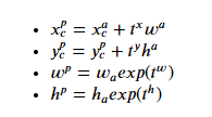
其中上标p表示区域建议,上标a表示锚框,t表示预测偏移。
以下函数实现上述转换并生成区域建议:
def generate_proposals(anchors, offsets):

    # change format of the anchor boxes from 'xyxy' to 'cxcywh'
    anchors = ops.box_convert(anchors, in_fmt='xyxy', out_fmt='cxcywh')

    # apply offsets to anchors to create proposals
    proposals_ = torch.zeros_like(anchors)
    proposals_[:,0] = anchors[:,0] + offsets[:,0]*anchors[:,2]
    proposals_[:,1] = anchors[:,1] + offsets[:,1]*anchors[:,3]
    proposals_[:,2] = anchors[:,2] * torch.exp(offsets[:,2])
    proposals_[:,3] = anchors[:,3] * torch.exp(offsets[:,3])

    # change format of proposals back from 'cxcywh' to 'xyxy'
    proposals = ops.box_convert(proposals_, in_fmt='cxcywh', out_fmt='xyxy')

    return proposals
区域建议网络
区域建议网络是检测器的第一阶段,它获取特征图并产生区域建议。
在这里,我们将主干网络、采样模块和建议模块组合成区域建议网络。
class RegionProposalNetwork(nn.Module):
    def __init__(self, img_size, out_size, out_channels):
        super().__init__()

        self.img_height, self.img_width = img_size
        self.out_h, self.out_w = out_size

        # downsampling scale factor
        self.width_scale_factor = self.img_width // self.out_w
        self.height_scale_factor = self.img_height // self.out_h

        # scales and ratios for anchor boxes
        self.anc_scales = [2, 4, 6]
        self.anc_ratios = [0.5, 1, 1.5]
        self.n_anc_boxes = len(self.anc_scales) * len(self.anc_ratios)

        # IoU thresholds for +ve and -ve anchors
        self.pos_thresh = 0.7
        self.neg_thresh = 0.3

        # weights for loss
        self.w_conf = 1
        self.w_reg = 5

        self.feature_extractor = FeatureExtractor()
        self.proposal_module = ProposalModule(out_channels, n_anchors=self.n_anc_boxes)

    def forward(self, images, gt_bboxes, gt_classes):
        batch_size = images.size(dim=0)
        feature_map = self.feature_extractor(images)

        # generate anchors
        anc_pts_x, anc_pts_y = gen_anc_centers(out_size=(self.out_h, self.out_w))
        anc_base = gen_anc_base(anc_pts_x, anc_pts_y, self.anc_scales, self.anc_ratios, (self.out_h, self.out_w))
        anc_boxes_all = anc_base.repeat(batch_size, 1, 1, 1, 1)

        # get positive and negative anchors amongst other things
        gt_bboxes_proj = project_bboxes(gt_bboxes, self.width_scale_factor, self.height_scale_factor, mode='p2a')

        positive_anc_ind, negative_anc_ind, GT_conf_scores, \
        GT_offsets, GT_class_pos, positive_anc_coords, \
        negative_anc_coords, positive_anc_ind_sep = get_req_anchors(anc_boxes_all, gt_bboxes_proj, gt_classes)

        # pass through the proposal module
        conf_scores_pos, conf_scores_neg, offsets_pos, proposals = self.proposal_module(feature_map, positive_anc_ind, \
                                                                                        negative_anc_ind, positive_anc_coords)

        cls_loss = calc_cls_loss(conf_scores_pos, conf_scores_neg, batch_size)
        reg_loss = calc_bbox_reg_loss(GT_offsets, offsets_pos, batch_size)

        total_rpn_loss = self.w_conf * cls_loss + self.w_reg * reg_loss

        return total_rpn_loss, feature_map, proposals, positive_anc_ind_sep, GT_class_pos

    def inference(self, images, conf_thresh=0.5, nms_thresh=0.7):
        with torch.no_grad():
            batch_size = images.size(dim=0)
            feature_map = self.feature_extractor(images)

            # generate anchors
            anc_pts_x, anc_pts_y = gen_anc_centers(out_size=(self.out_h, self.out_w))
            anc_base = gen_anc_base(anc_pts_x, anc_pts_y, self.anc_scales, self.anc_ratios, (self.out_h, self.out_w))
            anc_boxes_all = anc_base.repeat(batch_size, 1, 1, 1, 1)
            anc_boxes_flat = anc_boxes_all.reshape(batch_size, -1, 4)

            # get conf scores and offsets
            conf_scores_pred, offsets_pred = self.proposal_module(feature_map)
            conf_scores_pred = conf_scores_pred.reshape(batch_size, -1)
            offsets_pred = offsets_pred.reshape(batch_size, -1, 4)

            # filter out proposals based on conf threshold and nms threshold for each image
            proposals_final = []
            conf_scores_final = []
            for i in range(batch_size):
                conf_scores = torch.sigmoid(conf_scores_pred[i])
                offsets = offsets_pred[i]
                anc_boxes = anc_boxes_flat[i]
                proposals = generate_proposals(anc_boxes, offsets)
                # filter based on confidence threshold
                conf_idx = torch.where(conf_scores >= conf_thresh)[0]
                conf_scores_pos = conf_scores[conf_idx]
                proposals_pos = proposals[conf_idx]
                # filter based on nms threshold
                nms_idx = ops.nms(proposals_pos, conf_scores_pos, nms_thresh)
                conf_scores_pos = conf_scores_pos[nms_idx]
                proposals_pos = proposals_pos[nms_idx]

                proposals_final.append(proposals_pos)
                conf_scores_final.append(conf_scores_pos)

        return proposals_final, conf_scores_final, feature_map
在训练和推理过程中,RPN为所有锚框生成分数和偏移。然而,在训练期间,我们只选择正和负锚框来计算分类损失。为了计算L2回归损失,我们只考虑阳性样本的偏移。最终损失是这两种损失的加权组合。
在推断过程中,我们选择得分高于给定阈值的锚框,并使用预测的偏移量生成建议。我们使用S形函数将原始模型逻辑转换为概率分数。
在这两种情况下生成的建议被传递到检测器的第二阶段。
分类模块
在第二阶段,我们接收区域建议,并预测建议中对象的类别。这可以通过一个简单的卷积网络来实现,但有一个缺点:所有建议的大小都不相同。
现在,你可能会考虑在将建议输入模型之前调整大小,就像我们通常在图像分类任务中调整图像大小一样,但问题是调整大小不是一个可区分的操作,因此不能通过该操作进行反向传播。
这里有一个更聪明的调整大小的方法:我们将建议分成大致相等的子区域,并对每个子区域应用最大池操作,以产生相同大小的输出。这称为ROI池,如下所示:

最大池是一种可微操作,我们一直在卷积神经网络中使用它们。
我们不需要从头开始实施ROI池,torchvisio.ops库为我们提供了它。
一旦使用ROI池调整了建议的大小,我们将其通过卷积神经网络,该网络由卷积层、平均池层和产生类别分数的线性层组成。
在推理过程中,我们通过对原始模型逻辑应用softmax函数并选择具有最高概率得分的类别来预测对象类别。在训练期间,我们使用交叉熵计算分类损失。
class ClassificationModule(nn.Module):
    def __init__(self, out_channels, n_classes, roi_size, hidden_dim=512, p_dropout=0.3):
        super().__init__()
        self.roi_size = roi_size
        # hidden network
        self.avg_pool = nn.AvgPool2d(self.roi_size)
        self.fc = nn.Linear(out_channels, hidden_dim)
        self.dropout = nn.Dropout(p_dropout)

        # define classification head
        self.cls_head = nn.Linear(hidden_dim, n_classes)

    def forward(self, feature_map, proposals_list, gt_classes=None):

        if gt_classes is None:
            mode = 'eval'
        else:
            mode = 'train'

        # apply roi pooling on proposals followed by avg pooling
        roi_out = ops.roi_pool(feature_map, proposals_list, self.roi_size)
        roi_out = self.avg_pool(roi_out)

        # flatten the output
        roi_out = roi_out.squeeze(-1).squeeze(-1)

        # pass the output through the hidden network
        out = self.fc(roi_out)
        out = F.relu(self.dropout(out))

        # get the classification scores
        cls_scores = self.cls_head(out)

        if mode == 'eval':
            return cls_scores

        # compute cross entropy loss
        cls_loss = F.cross_entropy(cls_scores, gt_classes.long())

        return cls_loss
在一个全面的实现中,我们还将背景类别包括在第二阶段,但让我们将其留在本教程中。
在第二阶段,我们还添加了一个回归网络,该网络进一步为区域建议生成偏移量。然而,由于这需要额外的记录,我没有将其包含在本教程中。
非最大抑制
在推理的最后一步,我们使用一种称为非最大抑制的技术来删除重复的边界框。在该技术中,我们首先考虑具有最高分类分数的边界框。然后,我们用这个框计算所有其他框的IoU,并删除具有高IoU分数的框。这些是与“原始”边界框重叠的重复边界框。我们对剩余的框也重复此过程,直到删除所有重复项。
同样,我们不必从头开始实现它。torchvisio.ops库为我们提供了它。NMS处理步骤在上述第1阶段回归网络中实现。
Faster RCNN模型
我们将区域建议网络和分类模块结合起来,构建最终的端到端Faster RCNN模型。
class TwoStageDetector(nn.Module):
    def __init__(self, img_size, out_size, out_channels, n_classes, roi_size):
        super().__init__()
        self.rpn = RegionProposalNetwork(img_size, out_size, out_channels)
        self.classifier = ClassificationModule(out_channels, n_classes, roi_size)

    def forward(self, images, gt_bboxes, gt_classes):
        total_rpn_loss, feature_map, proposals, \
        positive_anc_ind_sep, GT_class_pos = self.rpn(images, gt_bboxes, gt_classes)

        # get separate proposals for each sample
        pos_proposals_list = []
        batch_size = images.size(dim=0)
        for idx in range(batch_size):
            proposal_idxs = torch.where(positive_anc_ind_sep == idx)[0]
            proposals_sep = proposals[proposal_idxs].detach().clone()
            pos_proposals_list.append(proposals_sep)

        cls_loss = self.classifier(feature_map, pos_proposals_list, GT_class_pos)
        total_loss = cls_loss + total_rpn_loss

        return total_loss

    def inference(self, images, conf_thresh=0.5, nms_thresh=0.7):
        batch_size = images.size(dim=0)
        proposals_final, conf_scores_final, feature_map = self.rpn.inference(images, conf_thresh, nms_thresh)
        cls_scores = self.classifier(feature_map, proposals_final)

        # convert scores into probability
        cls_probs = F.softmax(cls_scores, dim=-1)
        # get classes with highest probability
        classes_all = torch.argmax(cls_probs, dim=-1)

        classes_final = []
        # slice classes to map to their corresponding image
        c = 0
        for i in range(batch_size):
            n_proposals = len(proposals_final[i]) # get the number of proposals for each image
            classes_final.append(classes_all[c: c+n_proposals])
            c += n_proposals

        return proposals_final, conf_scores_final, classes_final
训练模型
首先,让我们在一小部分数据样本上拟合网络,以确保一切都按预期工作。我们使用Adam优化器的标准训练循环,学习率为1e-3。
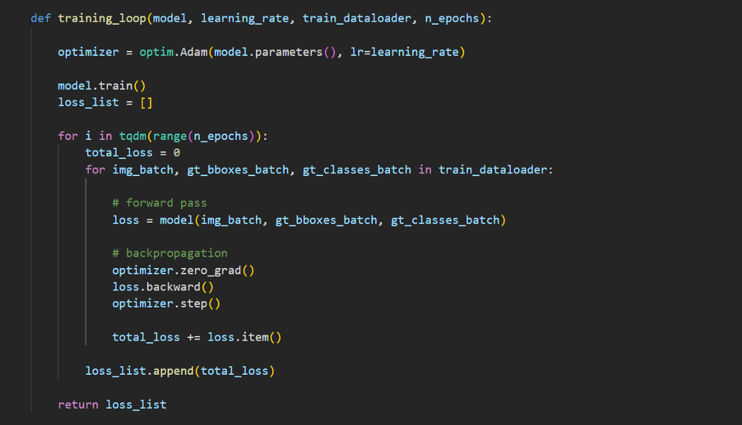
以下是结果:
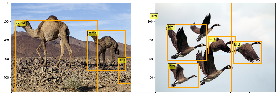
由于我们在一小部分数据上进行了训练,所以模型还没有学习到图像级别的特征,因此结果并不准确。这可以通过在大型数据集上进行训练来改善。
结论
在实现中,我们在标准数据集(如MS-COCO或PASCAL VOC)上训练网络,并使用平均精度或ROC曲线下面积等指标评估结果。然而,本教程的目的是了解Faster RCNN模型,因此我们将离开评估部分。
多年来,该领域取得了重大进展,并开发了许多新的网络。示例包括YOLO、EfficientDet、DETR和Mask RCNN。然而,它们中的大多数都建立在我们在本教程中讨论过的Faster RCNN模型所奠定的基础之上。
我希望你喜欢这篇文章。代码在GitHub中可用。
https://github.com/wingedrasengan927/pytorch-tutorials/tree/master/Object%20Detection
数据集
本文中使用的两幅图像来自DIV2K数据集。数据集在CC0:公共域下获得许可。
@InProceedings{Agustsson_2017_CVPR_Workshops,
 author = {Agustsson, Eirikur and Timofte, Radu},
 title = {NTIRE 2017 Challenge on Single Image Super-Resolution: Dataset and Study},
 booktitle = {The IEEE Conference on Computer Vision and Pattern Recognition (CVPR) Workshops},
 month = {July},
 year = {2017}
}
图像学分
除非标题中明确引用了源代码,否则本教程中的所有图像均由作者提供。
参考引用
Deep learning for Computer Vision, UMich(https://web.eecs.umich.edu/~justincj/teaching/eecs498/WI2022/)
Faster-RCNN paper(https://arxiv.org/abs/1506.01497)
☆ END ☆
如果看到这里,说明你喜欢这篇文章,请转发、点赞。微信搜索「uncle_pn」,欢迎添加小编微信「 woshicver」,每日朋友圈更新一篇高质量博文。
↓扫描二维码添加小编↓
