第二部分:sklearn分类实例
(一)、实例一:Gradient Boosting regression
Demonstrate Gradient Boosting on the Boston housing dataset.
This example fits a Gradient Boosting model with least squares loss and 500 regression trees of depth 4.
来源:点击打开链接
# Author: Peter Prettenhofer <[email protected]>
#
# License: BSD 3 clause

import numpy as np
import matplotlib.pyplot as plt

from sklearn import ensemble
from sklearn import datasets
from sklearn.utils import shuffle
from sklearn.metrics import mean_squared_error

# #############################################################################
# Load data
boston = datasets.load_boston()
X, y = shuffle(boston.data, boston.target, random_state=13)
X = X.astype(np.float32)
offset = int(X.shape[0] * 0.9)
X_train, y_train = X[:offset], y[:offset]
X_test, y_test = X[offset:], y[offset:]

# #############################################################################
# Fit regression model
params = {'n_estimators': 500, 'max_depth': 4, 'min_samples_split': 2,
          'learning_rate': 0.01, 'loss': 'ls'}
clf = ensemble.GradientBoostingRegressor(**params)

clf.fit(X_train, y_train)
mse = mean_squared_error(y_test, clf.predict(X_test))
print("MSE: %.4f" % mse)

# #############################################################################
# Plot training deviance

# compute test set deviance
test_score = np.zeros((params['n_estimators'],), dtype=np.float64)

for i, y_pred in enumerate(clf.staged_predict(X_test)):
    test_score[i] = clf.loss_(y_test, y_pred)

plt.figure(figsize=(12, 6))
plt.subplot(1, 2, 1)
plt.title('Deviance')
plt.plot(np.arange(params['n_estimators']) + 1, clf.train_score_, 'b-',
         label='Training Set Deviance')
plt.plot(np.arange(params['n_estimators']) + 1, test_score, 'r-',
         label='Test Set Deviance')
plt.legend(loc='upper right')
plt.xlabel('Boosting Iterations')
plt.ylabel('Deviance')

# #############################################################################
# Plot feature importance
feature_importance = clf.feature_importances_
# make importances relative to max importance
feature_importance = 100.0 * (feature_importance / feature_importance.max())
sorted_idx = np.argsort(feature_importance)
pos = np.arange(sorted_idx.shape[0]) + .5
plt.subplot(1, 2, 2)
plt.barh(pos, feature_importance[sorted_idx], align='center')
plt.yticks(pos, boston.feature_names[sorted_idx])
plt.xlabel('Relative Importance')
plt.title('Variable Importance')
plt.show()
结果如下所示:
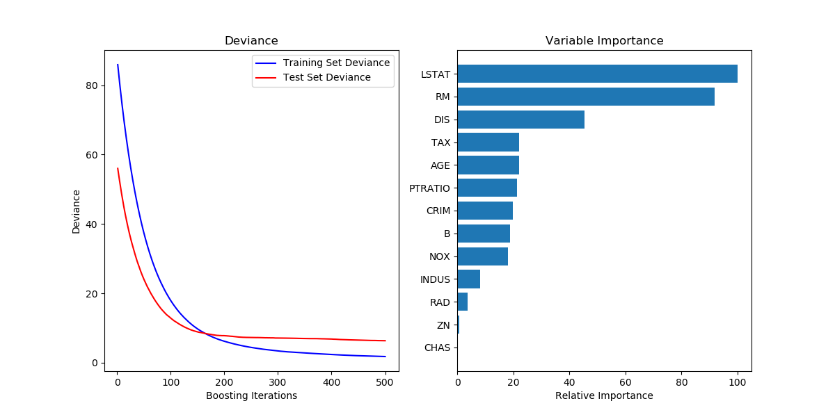
结果分析:从左图中可以看出,随着迭代次数的增加,Deviance这个值呈现出减小趋势直至逐渐稳定在大于0的某个值附近。而右图中的重要性分析中可以看到Lstat所占的重要性最高,最小的是CHAS。
存在的疑惑:不是很理解Deviance这个词的意思,查的是越轨,也有偏差之意,但是这里的值的数量级一开始甚至到了90,也许是百分比吧,以后弄清楚了再来补充。
实例二、Prediction Intervals for Gradient Boosting Regression基于梯度提升回归的区间预测
This example shows how quantile regression can be used to create prediction intervals.
"""
=====================================================
Prediction Intervals for Gradient Boosting Regression
=====================================================

This example shows how quantile regression can be used
to create prediction intervals.
"""

import numpy as np
import matplotlib.pyplot as plt
import time
from sklearn.ensemble import GradientBoostingRegressor

np.random.seed(1)


def f(x):
    """The function to predict."""
    return x * np.sin(x)

#----------------------------------------------------------------------
#  First the noiseless case
X = np.atleast_2d(np.random.uniform(0, 10.0, size=100)).T
X = X.astype(np.float32)

# Observations
y = f(X).ravel()  # numpy.ravel()返回的是视图(view),功能是将多维数组将为一维

dy = 1.5 + 1.0 * np.random.random(y.shape)
noise = np.random.normal(0, dy)
y += noise
y = y.astype(np.float32)

# Mesh the input space for evaluations of the real function, the prediction and
# its MSE
xx = np.atleast_2d(np.linspace(0, 10, 1000)).T
xx = xx.astype(np.float32)

alpha = 0.95   # 损失函数是quantile,alpha是其参数
startTime = time.time()
clf = GradientBoostingRegressor(loss='quantile', alpha=alpha,
                                n_estimators=250, max_depth=3,
                                learning_rate=.1, min_samples_leaf=9,
                                min_samples_split=9)

clf.fit(X, y)
print('---alpha=0.95 loss=quantile Training Completed.Took %f s.' % (time.time() - startTime))
# Make the prediction on the meshed x-axis
y_upper = clf.predict(xx)
startTime = time.time()
clf.set_params(alpha=1.0 - alpha)  # 这是两种预测,一种是在alpha=0.95时,一种是在alpha=0.05时
clf.fit(X, y)
print('---alpha=0.05 loss=quantile Training Completed.Took %f s.' % (time.time() - startTime))
# Make the prediction on the meshed x-axis
y_lower = clf.predict(xx)
startTime = time.time()
clf.set_params(loss='ls')   # 修改损失函数为ls 默认的最小二乘回归的
clf.fit(X, y)
print('---loss=ls Training Completed.Took %f s.' % (time.time() - startTime))
# Make the prediction on the meshed x-axis
y_pred = clf.predict(xx)

# Plot the function, the prediction and the 90% confidence interval based on
# the MSE
fig = plt.figure()
plt.plot(xx, f(xx), 'g:', label=u'$f(x) = x\,\sin(x)$')
plt.plot(X, y, 'b.', markersize=10, label=u'Observations')
plt.plot(xx, y_pred, 'r-', label=u'Prediction')
plt.plot(xx, y_upper, 'k-')
plt.plot(xx, y_lower, 'k-')
plt.fill(np.concatenate([xx, xx[::-1]]),
         np.concatenate([y_upper, y_lower[::-1]]),
         alpha=.5, fc='b', ec='None', label='90% prediction interval')
plt.xlabel('$x$')
plt.ylabel('$f(x)$')
plt.ylim(-10, 20)
plt.legend(loc='upper left')
plt.show()
输出结果如下:
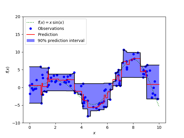
从代码中可以看出,在三种情况下拟合了回归学习器,包括alpha=0.95 loss=quantile,alpha=0.05 loss=quantile,loss=ls这三种模型,并且前两种得到了上图中的上下黑色的边界,中间用淡紫色填充;红色线是基于损失函数是最小二乘回归的情况下的预测值,可以看出还是比较符合观测值的,与f(x)的曲线也比较贴切。