GBDT分类实战完全总结(二)

第二部分：sklearn分类实例

实例一：Feature transformations with ensembles of trees使用集成树的特征转换

import numpy as np
np.random.seed(10)
# seed( ) 用于指定随机数生成时所用算法开始的整数值。
# 1.如果使用相同的seed( )值，则每次生成的随即数都相同；
# 2.如果不设置这个值，则系统根据时间来自己选择这个值，此时每次生成的随机数因时间差异而不同。
# 3.设置的seed()值仅一次有效

import matplotlib.pyplot as plt
import time
from sklearn.datasets import make_classification
from sklearn.linear_model import LogisticRegression
from sklearn.ensemble import (RandomTreesEmbedding, RandomForestClassifier,
                              GradientBoostingClassifier)
from sklearn.preprocessing import OneHotEncoder
from sklearn.model_selection import train_test_split
from sklearn.metrics import roc_curve
from sklearn.pipeline import make_pipeline

startTime = time.time()
print('Step 1.Prepareing data...')
n_estimator = 10         # 迭代次数
X, y = make_classification(n_samples=80000)   # 样本生成，这里生成了80000个样本
X_train, X_test, y_train, y_test = train_test_split(X, y, test_size=0.5)   # 将80000个样本分成一半是训练集，一半是测试集
# It is important to train the ensemble of trees on a different subset
# of the training data than the linear regression model to avoid
# overfitting, in particular if the total number of leaves is
# similar to the number of training samples
X_train, X_train_lr, y_train, y_train_lr = train_test_split(X_train,
                                                            y_train,
                                                            test_size=0.5)
print('Step 2.RT+LR...')
# Unsupervised transformation based on totally random trees
rt = RandomTreesEmbedding(max_depth=3, n_estimators=n_estimator,
	random_state=0)
# 逻辑回归
rt_lm = LogisticRegression()
pipeline = make_pipeline(rt, rt_lm)   # 构造函数 RT+LR
pipeline.fit(X_train, y_train)
y_pred_rt = pipeline.predict_proba(X_test)[:, 1]
fpr_rt_lm, tpr_rt_lm, _ = roc_curve(y_test, y_pred_rt)
print('Step 3.RF+LR...')
# Supervised transformation based on random forests
# 随机森林
rf = RandomForestClassifier(max_depth=3, n_estimators=n_estimator)
rf_enc = OneHotEncoder()
rf_lm = LogisticRegression()
rf.fit(X_train, y_train)
rf_enc.fit(rf.apply(X_train))
rf_lm.fit(rf_enc.transform(rf.apply(X_train_lr)), y_train_lr)

y_pred_rf_lm = rf_lm.predict_proba(rf_enc.transform(rf.apply(X_test)))[:, 1]    # RF+LR
fpr_rf_lm, tpr_rf_lm, _ = roc_curve(y_test, y_pred_rf_lm)

print('Step 4.GBT+LR...')
# 梯度提升决策树分类
grd = GradientBoostingClassifier(n_estimators=n_estimator)
grd_enc = OneHotEncoder()    # 数据预处理
grd_lm = LogisticRegression()
grd.fit(X_train, y_train)    # 训练GRD模型
grd_enc.fit(grd.apply(X_train)[:, :, 0])
grd_lm.fit(grd_enc.transform(grd.apply(X_train_lr)[:, :, 0]), y_train_lr)

y_pred_grd_lm = grd_lm.predict_proba(
    grd_enc.transform(grd.apply(X_test)[:, :, 0]))[:, 1]
fpr_grd_lm, tpr_grd_lm, _ = roc_curve(y_test, y_pred_grd_lm)   # 画ROC曲线，sklearn里面有相应的函数，横轴假正例率，纵轴真正例率；
# ROC曲线反映了分类器对正例的覆盖能力和对负例的覆盖能力之间的权衡。

print('Step 5.GBT...')
# The gradient boosted model by itself
y_pred_grd = grd.predict_proba(X_test)[:, 1]    # 单纯用提升树时的预测概率
fpr_grd, tpr_grd, _ = roc_curve(y_test, y_pred_grd)  # 得到绘制ROC曲线需要的fpr 和 tpr
print('Step 6.RF...')
# 随机森林预测
# The random forest model by itself
y_pred_rf = rf.predict_proba(X_test)[:, 1]
fpr_rf, tpr_rf, _ = roc_curve(y_test, y_pred_rf)
print('Step 7.Ploting...')
plt.figure(1)
plt.plot([0, 1], [0, 1], 'k--')
plt.plot(fpr_rt_lm, tpr_rt_lm, label='RT + LR')
plt.plot(fpr_rf, tpr_rf, label='RF')
plt.plot(fpr_rf_lm, tpr_rf_lm, label='RF + LR')
plt.plot(fpr_grd, tpr_grd, label='GBT')
plt.plot(fpr_grd_lm, tpr_grd_lm, label='GBT + LR')
plt.xlabel('False positive rate')
plt.ylabel('True positive rate')
plt.title('ROC curve')
plt.legend(loc='best')
plt.show()
print('Step 8.局部放大图...')
plt.figure(2)
plt.xlim(0, 0.2)
plt.ylim(0.8, 1)
plt.plot([0, 1], [0, 1], 'k--')
plt.plot(fpr_rt_lm, tpr_rt_lm, label='RT + LR')
plt.plot(fpr_rf, tpr_rf, label='RF')
plt.plot(fpr_rf_lm, tpr_rf_lm, label='RF + LR')
plt.plot(fpr_grd, tpr_grd, label='GBT')
plt.plot(fpr_grd_lm, tpr_grd_lm, label='GBT + LR')
plt.xlabel('False positive rate')
plt.ylabel('True positive rate')
plt.title('ROC curve (zoomed in at top left)')
plt.legend(loc='best')
plt.show()
print('---Training Completed.Took %f s.' % (time.time() - startTime))

输出结果如下：

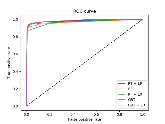
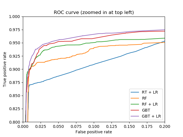
图中输出的是这五种方法的ROC曲线对比图，ROC曲线反映了分类器对正例的覆盖能力和对负例的覆盖能力之间的权衡，从图中可以看出GBT+LR有着最高的真正例率曲线值，依次往上，真正例率值依次降低。

按照ROC曲线的性质，如果一个学习器的ROC曲线被另一个学习器的ROC曲线完全“包住”，那么可以断言后者的性能优于前者，如果两者有相交，则需要对比各自的覆盖面积。

若按照是否包裹来论，GBT+LR基本上可以包住其他四个的曲线，但是在最前面有所交叉，因此不能完全断言所有的关系；若按照覆盖面积来论，GBT+LR的覆盖面积最大，之后依次是GBT,RF+LR,RF,RT+LR，那么对应的性能从优到劣依次为：GBT+LR>GBT>RF+LR>RF>RT+LR。

实例二：Gradient Boosting Out-of-Bag estimates

参考： 点击打开链接

名词：out of bag（the improvement in loss based on the examples not included in the bootstrap sample对损失函数的改进是基于非自助法抽样的样本）

OOB估计是一种有用且具有启发性的估计最优迭代次数的方法，它等价于交叉验证法，但具有实时（on-the -fly）计算不需要反复拟合模型。OOB只适用于随机梯度提升（即子样本个数<1,也就是说没有子样本，应该说它是每个基训练器树属性分割最优的参数结果的训练器）。OOB分类器是对真实的测试集的悲观估计，但仍然保留了小样本（未被bootstrap选中的）决策树的比较好的近似估计。

# Author: Peter Prettenhofer <[email protected]>
#
# License: BSD 3 clause

import numpy as np
import matplotlib.pyplot as plt

from sklearn import ensemble
from sklearn.model_selection import KFold
from sklearn.model_selection import train_test_split


# Generate data (adapted from G. Ridgeway's gbm example)
n_samples = 1000
random_state = np.random.RandomState(13)
x1 = random_state.uniform(size=n_samples)   # 产生1行1000列的assarray，其中的每个元素都是[0,1]区间的均匀分布的随机数
x2 = random_state.uniform(size=n_samples)
x3 = random_state.randint(0, 4, size=n_samples)  # 产生1行1000列的assarray，其中的每个元素都是[0,4]区间的均匀分布的随机数

p = 1 / (1.0 + np.exp(-(np.sin(3 * x1) - 4 * x2 + x3)))
y = random_state.binomial(1, p, size=n_samples)   # 二项分布，1次实验p的概率成果，重复1000次

X = np.c_[x1, x2, x3]  # 按行连接两个矩阵，就是把两矩阵左右相加，要求行数相等

X = X.astype(np.float32)
X_train, X_test, y_train, y_test = train_test_split(X, y, test_size=0.5,
                                                    random_state=9)

# Fit classifier with out-of-bag estimates
params = {'n_estimators': 1200, 'max_depth': 3, 'subsample': 0.5,
          'learning_rate': 0.01, 'min_samples_leaf': 1, 'random_state': 3}
clf = ensemble.GradientBoostingClassifier(**params)

clf.fit(X_train, y_train)
acc = clf.score(X_test, y_test)
print("Accuracy: {:.4f}".format(acc))  # 损失函数误差值y

n_estimators = params['n_estimators']
x = np.arange(n_estimators) + 1


def heldout_score(clf, X_test, y_test):
    """compute deviance scores on ``X_test`` and ``y_test``. """
    score = np.zeros((n_estimators,), dtype=np.float64)
    for i, y_pred in enumerate(clf.staged_decision_function(X_test)):
        score[i] = clf.loss_(y_test, y_pred)
    return score  # 每一个基分类器的损失函数值组成的数组


def cv_estimate(n_splits=3):
    cv = KFold(n_splits=n_splits)
    cv_clf = ensemble.GradientBoostingClassifier(**params)
    val_scores = np.zeros((n_estimators,), dtype=np.float64)
    for train, test in cv.split(X_train, y_train):
        cv_clf.fit(X_train[train], y_train[train])
        val_scores += heldout_score(cv_clf, X_train[test], y_train[test])
    val_scores /= n_splits
    return val_scores  # 求损失函数平均分


# Estimate best n_estimator using cross-validation
cv_score = cv_estimate(3)

# Compute best n_estimator for test data
test_score = heldout_score(clf, X_test, y_test)  # 测试集的评分

# negative cumulative sum of oob improvements
cumsum = -np.cumsum(clf.oob_improvement_)  # 一次都没抽到的训练集（最悲观情况的样本）的损失误差值的累加和

# min loss according to OOB
oob_best_iter = x[np.argmin(cumsum)]

# min loss according to test (normalize such that first loss is 0)
test_score -= test_score[0]  # 对损失函数值标准化，即令第一个基分类器损失值标准化0
test_best_iter = x[np.argmin(test_score)]

# min loss according to cv (normalize such that first loss is 0)
cv_score -= cv_score[0]
cv_best_iter = x[np.argmin(cv_score)]

# color brew for the three curves
oob_color = list(map(lambda x: x / 256.0, (190, 174, 212)))
test_color = list(map(lambda x: x / 256.0, (127, 201, 127)))
cv_color = list(map(lambda x: x / 256.0, (253, 192, 134)))

# plot curves and vertical lines for best iterations
plt.plot(x, cumsum, label='OOB loss', color=oob_color)
plt.plot(x, test_score, label='Test loss', color=test_color)
plt.plot(x, cv_score, label='CV loss', color=cv_color)
plt.axvline(x=oob_best_iter, color=oob_color)  # 画一条垂直线，x为位置，color为线的颜色
plt.axvline(x=test_best_iter, color=test_color)
plt.axvline(x=cv_best_iter, color=cv_color)

# add three vertical lines to xticks
xticks = plt.xticks()  # plt.xticks()返回x轴的刻度值、标签名
xticks_pos = np.array(xticks[0].tolist() +
                      [oob_best_iter, cv_best_iter, test_best_iter])  # 添加x轴刻度值
xticks_label = np.array(list(map(lambda t: int(t), xticks[0])) +
                        ['OOB', 'CV', 'Test'])  # 添加x轴标签名
ind = np.argsort(xticks_pos)  # 对刻度值从小到大排序，返回排序后的索引值
xticks_pos = xticks_pos[ind]  # 从小到大的刻度值
xticks_label = xticks_label[ind]  # 从小到大的标签名
plt.xticks(xticks_pos, xticks_label)  # 设置刻度值、标签名

plt.legend(loc='upper right')  # 设置图例位置
plt.ylabel('normalized loss')
plt.xlabel('number of iterations')

plt.show()

运行结果如下：

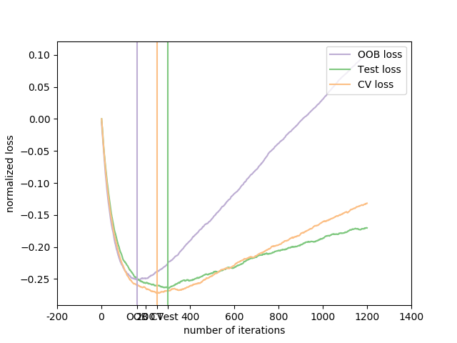
横轴为迭代次数，纵轴为归一化损失值，图例分别是：使用交叉验证来估计损失，测试集的损失，OOB损失。

图中共有六条线，其中的三条直线是三种估计方法所取得的归一化损失的最小值，用各自的颜色划一直线表示；三条曲线表示这三种估计方法对测试集的损失值随着迭代次数的增加，基本趋势是先减少后增大，这表明：迭代次数并非越大越好。

实例三、Gradient Boosting regularization-----梯度提升正则化

Illustration of the effect of different regularization strategies for Gradient Boosting. The example is taken from Hastie et al 2009 [1].

The loss function used is binomial deviance. Regularization via shrinkage (learning_rate < 1.0) improves performance considerably. In combination with shrinkage, stochastic gradient boosting (subsample < 1.0) can produce more accurate models by reducing the variance via bagging. Subsampling without shrinkage usually does poorly. Another strategy to reduce the variance is by subsampling the features analogous to the random splits in Random Forests (via the max_features parameter).

[1] T. Hastie, R. Tibshirani and J. Friedman, “Elements of Statistical Learning Ed. 2”, Springer, 2009.

正则化regularization

• Shrinkage：即学习率

v就是学习率。 一般情况下,越小的学习率,可以越好的逼近预测值,不容易产生过拟合，迭代次数会增加,经验上一般选取0.1左右。

• 使用缩减训练集

Friedman提出在每次迭代时对base learner从原始训练集中随机抽取一部分（a subsample of the training set drawn at random without replacement）作为本次base learner去拟合的样本集可以提高算法最后的准确率。

# Author: Peter Prettenhofer <[email protected]>
#
# License: BSD 3 clause

import numpy as np
import matplotlib.pyplot as plt

from sklearn import ensemble
from sklearn import datasets


X, y = datasets.make_hastie_10_2(n_samples=12000, random_state=1)
X = X.astype(np.float32)

# map labels from {-1, 1} to {0, 1}
labels, y = np.unique(y, return_inverse=True)

X_train, X_test = X[:2000], X[2000:]
y_train, y_test = y[:2000], y[2000:]

original_params = {'n_estimators': 1000, 'max_leaf_nodes': 4, 'max_depth': None, 'random_state': 2,
                   'min_samples_split': 5}

plt.figure()

for label, color, setting in [('No shrinkage', 'orange',
                               {'learning_rate': 1.0, 'subsample': 1.0}),
                              ('learning_rate=0.1', 'turquoise',
                               {'learning_rate': 0.1, 'subsample': 1.0}),
                              ('subsample=0.5', 'blue',
                               {'learning_rate': 1.0, 'subsample': 0.5}),
                              ('learning_rate=0.1, subsample=0.5', 'gray',
                               {'learning_rate': 0.1, 'subsample': 0.5}),
                              ('learning_rate=0.1, max_features=2', 'magenta',
                               {'learning_rate': 0.1, 'max_features': 2})]:
    params = dict(original_params)
    params.update(setting)

    clf = ensemble.GradientBoostingClassifier(**params)
    clf.fit(X_train, y_train)

    # compute test set deviance
    test_deviance = np.zeros((params['n_estimators'],), dtype=np.float64)

    for i, y_pred in enumerate(clf.staged_decision_function(X_test)):
        # clf.loss_ assumes that y_test[i] in {0, 1}
        test_deviance[i] = clf.loss_(y_test, y_pred)

    plt.plot((np.arange(test_deviance.shape[0]) + 1)[::5], test_deviance[::5],
            '-', color=color, label=label)

plt.legend(loc='upper left')
plt.xlabel('Boosting Iterations')
plt.ylabel('Test Set Deviance')

plt.show()

结果如下所示：

其对应的训练时间为：

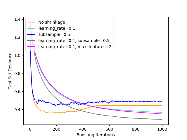
横坐标是Boosting迭代次数，纵坐标是测试集偏差，从图中可以看出：

（1）当不采用收缩学习时，黄色曲线下降最快，表明可以在较少的迭代次数达到较好的偏差效果，但是随着迭代次数增加，其偏差反而会增大一部分，继而稳定；

（2）其次是蓝色曲线，子采样为0.5（如果小于1.0，则会导致随机梯度增强），同样是下降最快，但是与黄色曲线相比，蓝色线最后稳定在一个值附近，这个值比黄色线要大。

（3）其余三条曲线趋势类似，其中最好的是灰色曲线，即learning_rate=0.1, subsample=0.5时，下降趋势在三条曲线中是最快的，并且其测出的偏差一直处于较小的值。

（4）五种情况下，训练时间的情况是：青色>灰色>蓝色>黄色>玫红色；

因此得到结论：如果想在较短的时间和较少的迭代次数情况下得到较好的性能，选择黄色No shrinkage，如果不考虑时间和迭代次数，只需要性能最好，选择灰色曲线代表的方法，即learning_rate=0.1, subsample=0.5。

That's all............