时间序列分析——基于R | 第2章 时间序列的预处理习题
1.考虑序列{1,2,3,4,5,…,20}
1.1判断该序列是否平稳
x <- seq(1,20);x## [1] 1 2 3 4 5 6 7 8 9 10 11 12 13 14 15 16 17 18 19 201.2样本自相关系数
max_lag <- 6
acf_x <- acf(x, lag.max = max_lag, plot = FALSE)$acf
r_1_to_6 <- acf_x[2:(max_lag + 1)] ;r_1_to_6
## [1] 0.8500000 0.7015038 0.5560150 0.4150376 0.2800752 0.1526316# 注意要从第2个元素开始提取,因为acf函数的结果向量的第一个元素对应滞后期数为0的自相关系数。1.3序列自相关图
#加载必要的包
library(ggplot2)
library(ggfortify)
library(RColorBrewer)
library(forecast)
#设置颜色主题
my_palette <- brewer.pal(n = 8, name = "Dark2")
#绘制序列自相关图并美化
windowsFonts(myFont = windowsFont("思源宋体 SemiBold"))
ggAcf(x) +
ggtitle("序列自相关图") + #添加标题
xlab("滞后") + #添加x轴标签
ylab("自相关系数") + #添加y轴标签
theme_minimal(base_size = 12, base_family = 'myFont') +
theme(plot.title = element_text(hjust = 0.5), #居中标题
panel.grid.minor = element_blank(), #去除次要网格线
panel.grid.major.x = element_line(size = 0.2, linetype = "dashed", color = "grey70"), #设置x轴主要网格线样式
axis.line.x = element_line(size = 0.5, color = "black"), #设置x轴线条粗细和颜色
axis.line.y = element_line(size = 0.5, color = "black"), #设置y轴线条粗细和颜色
axis.text = element_text(size = 10, color = my_palette[1]), #设置刻度标签字体大小和颜色
axis.title = element_text(size = 12, face = "bold", color = my_palette[2]), #设置轴标题字体大小、加粗和颜色
panel.border = element_blank(), #去除面板边框
panel.background = element_blank(), #去除面板背景
legend.background = element_blank(), #去除图例背景
legend.title = element_blank(), #去除图例标题
legend.text = element_text(size = 10, color = my_palette[3]), #设置图例文本字体大小和颜色
legend.position = c(0.9, 0.8)) + #设置图例位置
scale_color_manual(values = my_palette[4:8]) #设置线条颜色
2.1975-1980年夏威夷岛莫那罗亚火山每月释放的CO₂数据
2.1绘制时序图,判断平稳性
d2=c(t(read.table('./时间序列分析——基于R(第2版)习题数据/习题2.2数据.txt', sep = '\t')))
ts_d2 <- ts(d2, start = c(1975,1), frequency = 12);ts_d2
## Jan Feb Mar Apr May Jun Jul Aug Sep Oct
## 1975 330.45 330.97 331.64 332.87 333.61 333.55 331.90 330.05 328.58 328.31
## 1976 331.63 332.46 333.36 334.45 334.82 334.32 333.05 330.87 329.24 328.87
## 1977 332.81 333.23 334.55 335.82 336.44 335.99 334.65 332.41 331.32 330.73
## 1978 334.66 335.07 336.33 337.39 337.65 337.57 336.25 334.39 332.44 332.25
## 1979 335.89 336.44 337.63 338.54 339.06 338.95 337.41 335.71 333.68 333.69
## 1980 337.81 338.16 339.88 340.57 341.19 340.87 339.25 337.19 335.49 336.63
## Nov Dec
## 1975 329.41 330.63
## 1976 330.18 331.50
## 1977 332.05 333.53
## 1978 333.59 334.76
## 1979 335.05 336.53
## 1980 337.74 338.36#加载必要的包library(ggplot2)
library(ggfortify)
library(RColorBrewer)
library(forecast)
# 绘制时序图
windowsFonts(myFont = windowsFont("思源宋体 SemiBold"))
ggplot() +
geom_line(aes(x = time(ts_d2), y = ts_d2),
color = "#74759b", size = 1.2) +
labs(title = "Monthly CO2 Emissions from Mauna Loa, Hawaii, 1975-1980",
x = "Year", y = "CO2 Emissions") +
theme_minimal(base_size = 12, base_family = 'myFont') +
theme(plot.title = element_text(face = "bold"),
axis.title = element_text(face = "bold", colour = '#132c33'),
axis.line = element_line(size = 0.75, colour = '#2b73af'),
axis.ticks = element_line(size = 0.5, colour = '#2376b7'),
panel.grid.major = element_blank(),
panel.grid.minor = element_blank())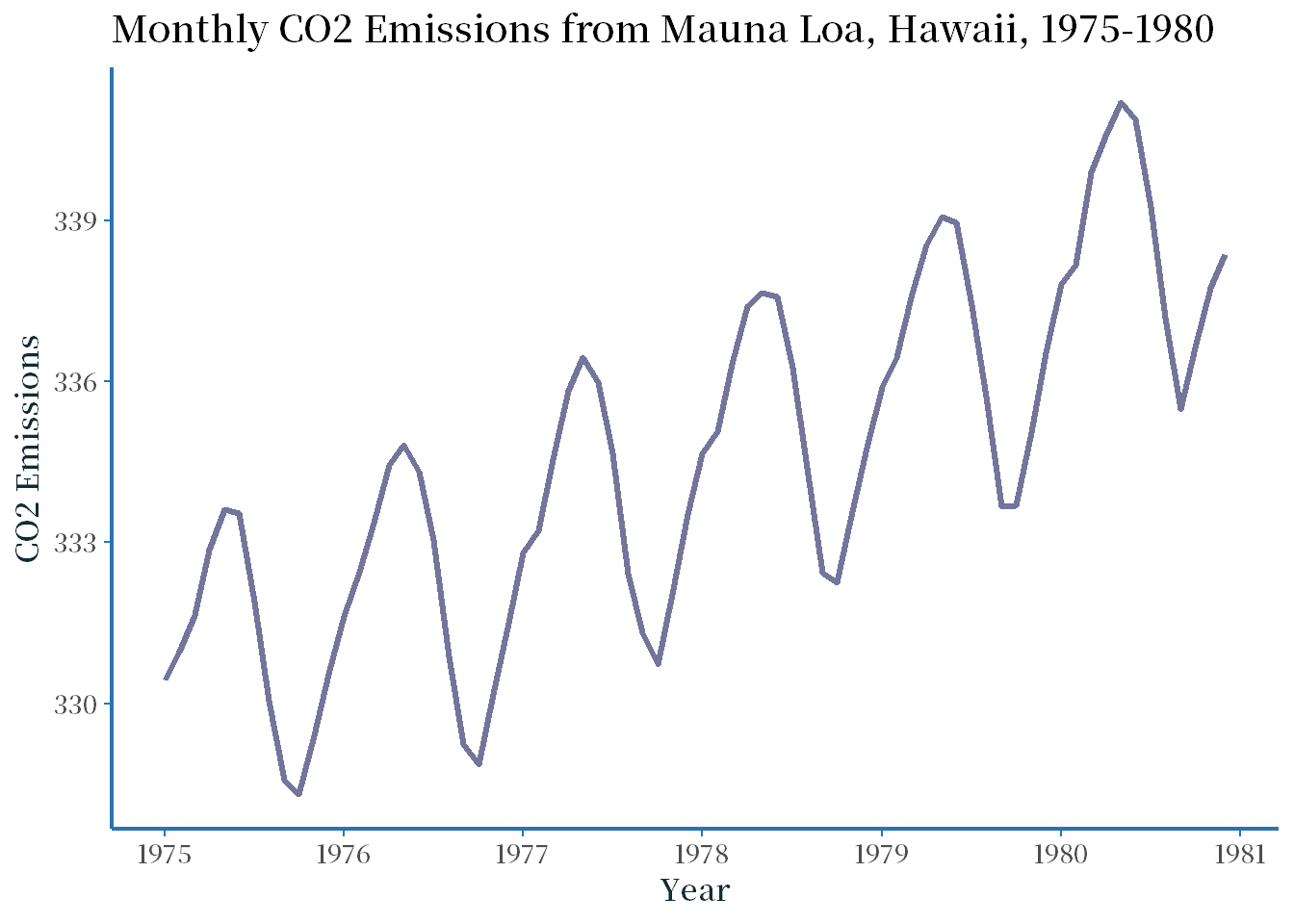
从时序图中可以看出,该序列存在较明显的季节性,同时也存在一定的趋势性。
2.2计算样本自相关系数
max_lag1 <- 24
acf_d2ts <- acf(ts_d2, lag.max = max_lag1, plot = FALSE)$acf
acf_d2ts[2:(max_lag1 + 1)]
## [1] 0.90750778 0.72171377 0.51251814 0.34982244 0.24689637 0.20309427
## [7] 0.21020799 0.26428810 0.36433219 0.48471672 0.58456166 0.60197891
## [13] 0.51841257 0.36856286 0.20671211 0.08138070 0.00135460 -0.03247916
## [19] -0.02709893 0.01123597 0.08274806 0.17010715 0.24319854 0.252522942.3绘制自相关图
ggAcf(ts_d2, lag.max = 36) +
  theme_minimal(base_size = 10, base_family = "myFont") +
  theme(plot.title = element_text(face = "bold", size = 14, hjust = 0.5),
        axis.title = element_text(face = "bold", hjust = 0.5),
        panel.grid.major = element_blank(),
        panel.grid.minor = element_blank(),
        axis.line = element_line(size = 0.75),
        axis.ticks = element_line(size = 0.5),
        axis.text = element_text(size = 12, color = "#815c94"),
        strip.text = element_text(size = 12, color = "#815c94", face = "bold"))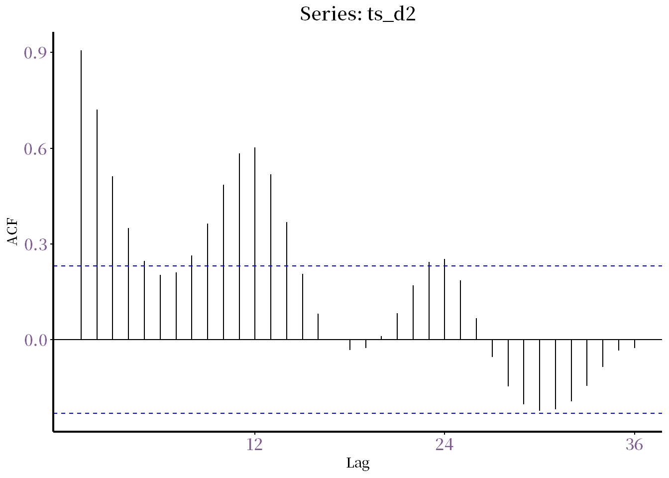
从自相关图中可以看出,该序列存在较强的季节性和自相关性,不具有平稳性。
3.1945-1950年费城月度降雨量数据
3.1样本自相关系数
d3 <- c(t(read.table('./时间序列分析——基于R(第2版)习题数据/习题2.3数据.txt', sep = '\t')));
ts_d3 <- ts(d3, start = c(1945,1), frequency = 12);ts_d3
## Jan Feb Mar Apr May Jun Jul Aug Sep Oct Nov Dec
## 1945 69.3 80.0 40.9 74.9 84.6 101.1 225.0 95.3 100.6 48.3 144.5 28.3
## 1946 38.4 52.3 68.6 37.1 148.6 218.7 131.6 112.8 81.8 31.0 47.5 70.1
## 1947 96.8 61.5 55.6 171.7 220.5 119.4 63.2 181.6 73.9 64.8 166.9 48.0
## 1948 137.7 80.5 105.2 89.9 174.8 124.0 86.4 136.9 31.5 35.3 112.3 43.0
## 1949 160.8 97.0 80.5 62.5 158.2 7.6 165.9 106.7 92.2 63.2 26.2 77.0
## 1950 52.3 105.4 144.3 49.5 116.1 54.1 148.6 159.3 85.3 67.3 112.8 59.4max_lag2 <- 24
acf_d3 <- acf(ts_d3, lag.max = max_lag2, plot = FALSE)$acf
acf_d3[2:(max_lag1 + 1)] ## [1] 0.012770216 0.041600613 -0.043230426 -0.178692841 -0.251298873
## [6] -0.093810241 -0.067777725 -0.071978515 0.013882228 0.109450351
## [11] 0.217295088 0.315872697 -0.025053744 0.075320665 -0.141206897
## [16] -0.203589406 -0.245494618 0.066461869 -0.139454035 -0.034028373
## [21] 0.205723132 -0.009866008 0.080311638 0.1180561903.2判断平稳性
#加载必要的包library(ggplot2)
library(ggfortify)
library(RColorBrewer)
library(forecast)

# 绘制时序图
ggplot(data = ts_d3, aes(x = seq_along(ts_d3), y = ts_d3)) +
  geom_line(color = "#0072B2", size = 1.2) +
  labs(x = "Time", y = "Monthly Precipitation (mm)",
       title = "Monthly Precipitation in Philadelphia, 1945-1950") +
  theme_minimal(base_size = 14, base_family = "myFont") +
  theme(plot.title = element_text(face = "bold", size = 14, hjust = 0.5),
        axis.text = element_text(size = 12, color = "#0072B2"),
        axis.title = element_text(size = 12, face = "bold", color = "#0072B2"))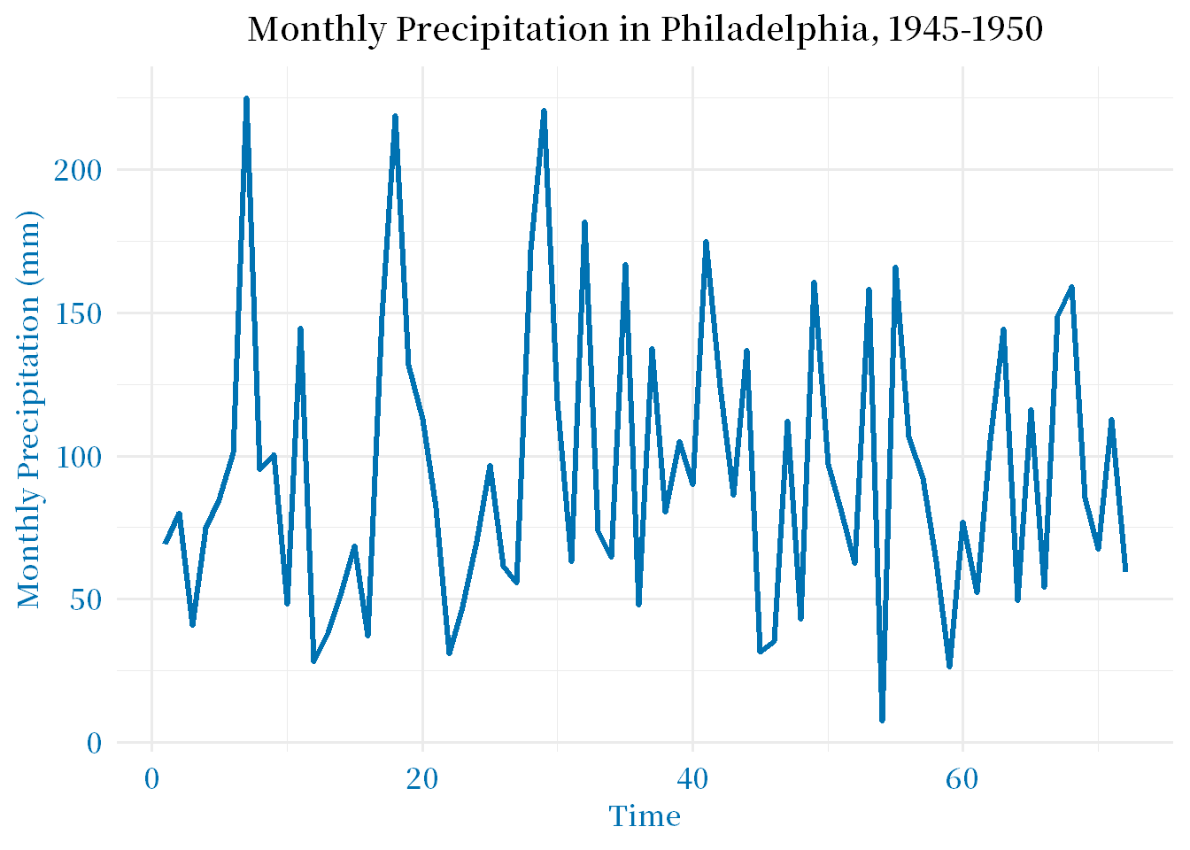
# 绘制自相关图
ggAcf(ts_d3, lag.max = 24) +
  theme_minimal(base_size = 14, base_family = "myFont") +
  theme(plot.title = element_text(face = "bold", size = 14, hjust = 0.5),
        axis.text = element_text(size = 12, color = "#0072B2"),
        axis.title = element_text(size = 12, face = "bold", color = "#0072B2"))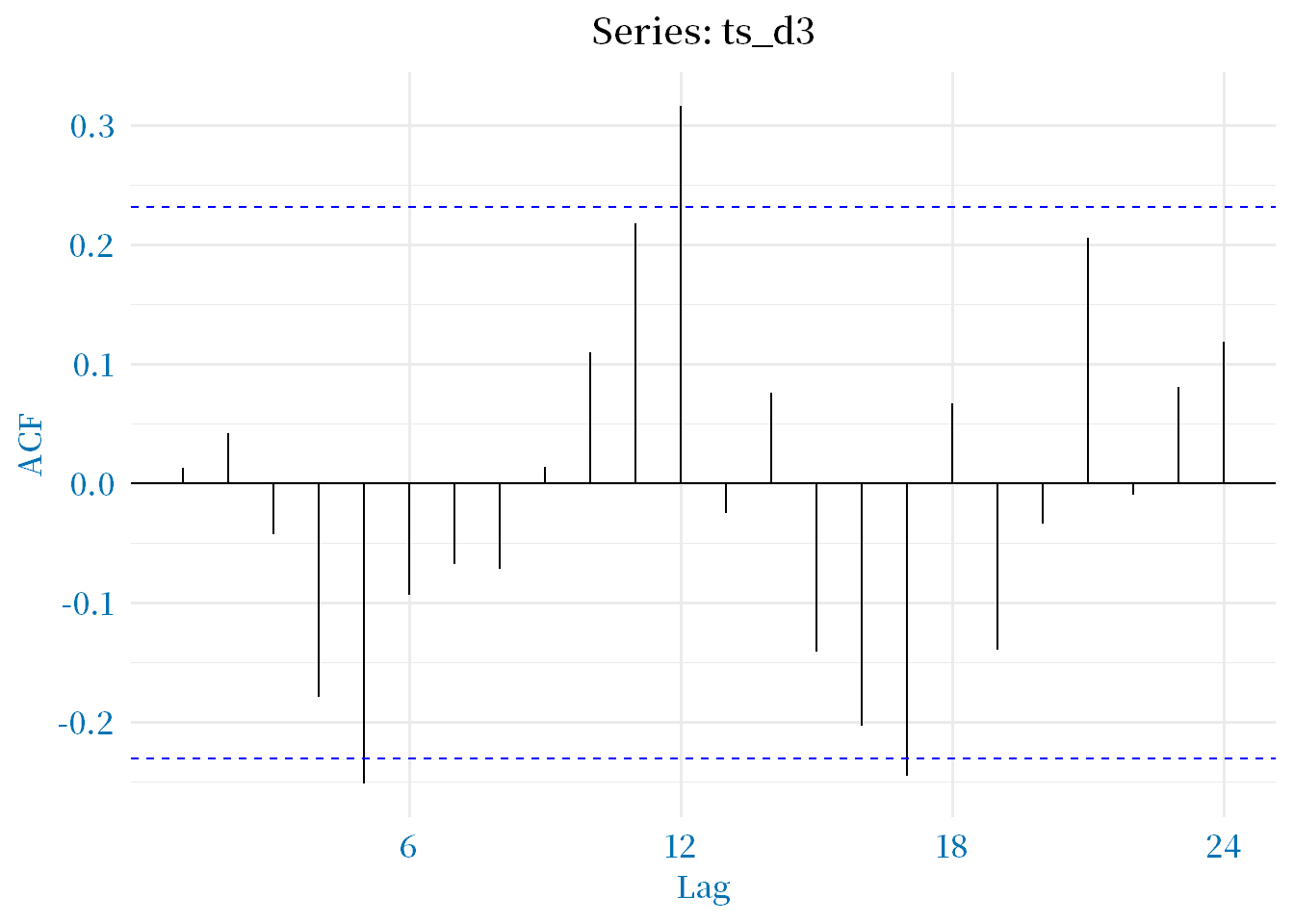
时序图显示了该数据集的所有观察值,其中每个点代表一个月的降雨量。我们可以看到,该序列具有一些季节性,但没有明显的趋势或周期性。
自相关图显示了每个滞后时点的自相关系数。我们可以看到,自相关系数在较短的滞后期内很高,随着滞后期的增加而逐渐降低。这表明该序列具有一些自相关性,但可能不是非常平稳。
3.3判断随机性
for (k in1:3) print(Box.test(d3, lag = 6*k, type = 'Ljung-Box'))##
## Box-Ljung test
##
## data: d3
## X-squared = 8.5225, df = 6, p-value = 0.2023
##
##
## Box-Ljung test
##
## data: d3
## X-squared = 23.36, df = 12, p-value = 0.02482
##
##
## Box-Ljung test
##
## data: d3
## X-squared = 36.02, df = 18, p-value = 0.007015#白噪声序列4.判断序列是否为纯随机序列(ɑ=0.05)
# 假设前12个样本的自相关系数存储在一个名为 acf_x 的向量中
acf_x <- c(0.02, 0.05, 0.10, -0.02, 0.05, 0.01, 0.12, -0.06, 0.08, -0.05, 0.02, -0.05)

# 假设最大滞后阶数为10
max_lag <- 10# 计算样本自相关系数的标准误
se <- 1/sqrt(100)

# 计算Ljung-Box检验的统计量和临界值
lb_stat <- sum((acf_x[-1])^2/(1:length(acf_x[-1])))/100/(se^2)
lb_crit <- qchisq(0.95, max_lag)

# 判断序列是否为纯随机序列if (lb_stat < lb_crit) {
  cat("序列可能是纯随机序列")
} else {
  cat("序列不是纯随机序列")
}
## 序列可能是纯随机序列5.某公司在2000-2003年间每月的销售量
5.1绘制时序图和样本自相关图
d5 <- read.table('./时间序列分析——基于R(第2版)习题数据/习题2.5数据.txt', header = TRUE);d5## 月份 X2000年 X2001年 X2002年 X2003年
## 1 1月 153 134 145 117
## 2 2月 187 175 203 178
## 3 3月 234 243 189 149
## 4 4月 212 227 214 178
## 5 5月 300 298 295 248
## 6 6月 221 256 220 202
## 7 7月 201 237 231 162
## 8 8月 175 165 174 135
## 9 9月 123 124 119 120
## 10 10月 104 106 85 96
## 11 11月 85 87 67 90
## 12 12月 78 74 75 63ts_d5 <- ts(c(d5$X2000年, d5$X2001年, d5$X2002年, d5$X2003年),
start = c(2000, 1), frequency = 12);ts_d5## Jan Feb Mar Apr May Jun Jul Aug Sep Oct Nov Dec
## 2000 153 187 234 212 300 221 201 175 123 104 85 78
## 2001 134 175 243 227 298 256 237 165 124 106 87 74
## 2002 145 203 189 214 295 220 231 174 119 85 67 75
## 2003 117 178 149 178 248 202 162 135 120 96 90 63#加载必要的包library(ggplot2)
library(ggfortify)
library(RColorBrewer)
library(forecast)
# 绘制时序图
ggplot(data = ts_d5, aes(x = seq_along(ts_d5), y = ts_d5)) +
geom_line(color = "#5d3131", size = 1.2) +
labs(x = "时间", y = "销售量",
title = "销售量时序图") +
theme_minimal(base_size = 14, base_family = "myFont") +
theme(plot.title = element_text(face = "bold", size = 14, hjust = 0.5),
axis.line = element_line(size = 0.5, colour = '#ed3333'),
axis.ticks = element_line(size = 0.5, colour = '#ed3333'),
axis.text = element_text(size = 12, color = "#daa45a"),
axis.title = element_text(size = 12, face = "bold", color = "#5d3131"))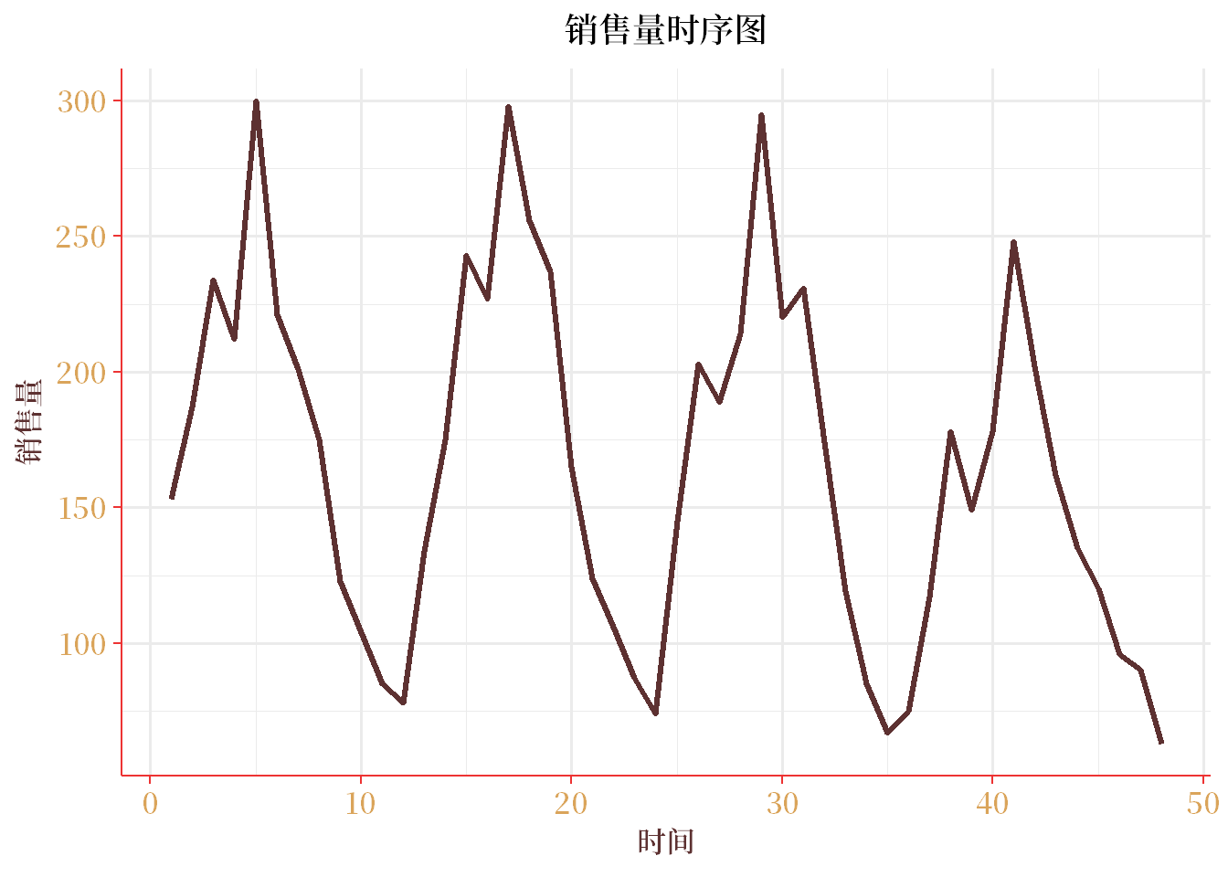
# 绘制自相关图
ggAcf(ts_d5, lag.max = 12) +
  labs(title = "Sample Autocorrelation Function", x = "Lag", y = "Autocorrelation") +
  theme_minimal() +
  theme(plot.title = element_text(size = 18, face = "bold", hjust = 0.5),
        axis.title = element_text(size = 14, face = "bold"),
        axis.text = element_text(size = 12),
        legend.position = "none")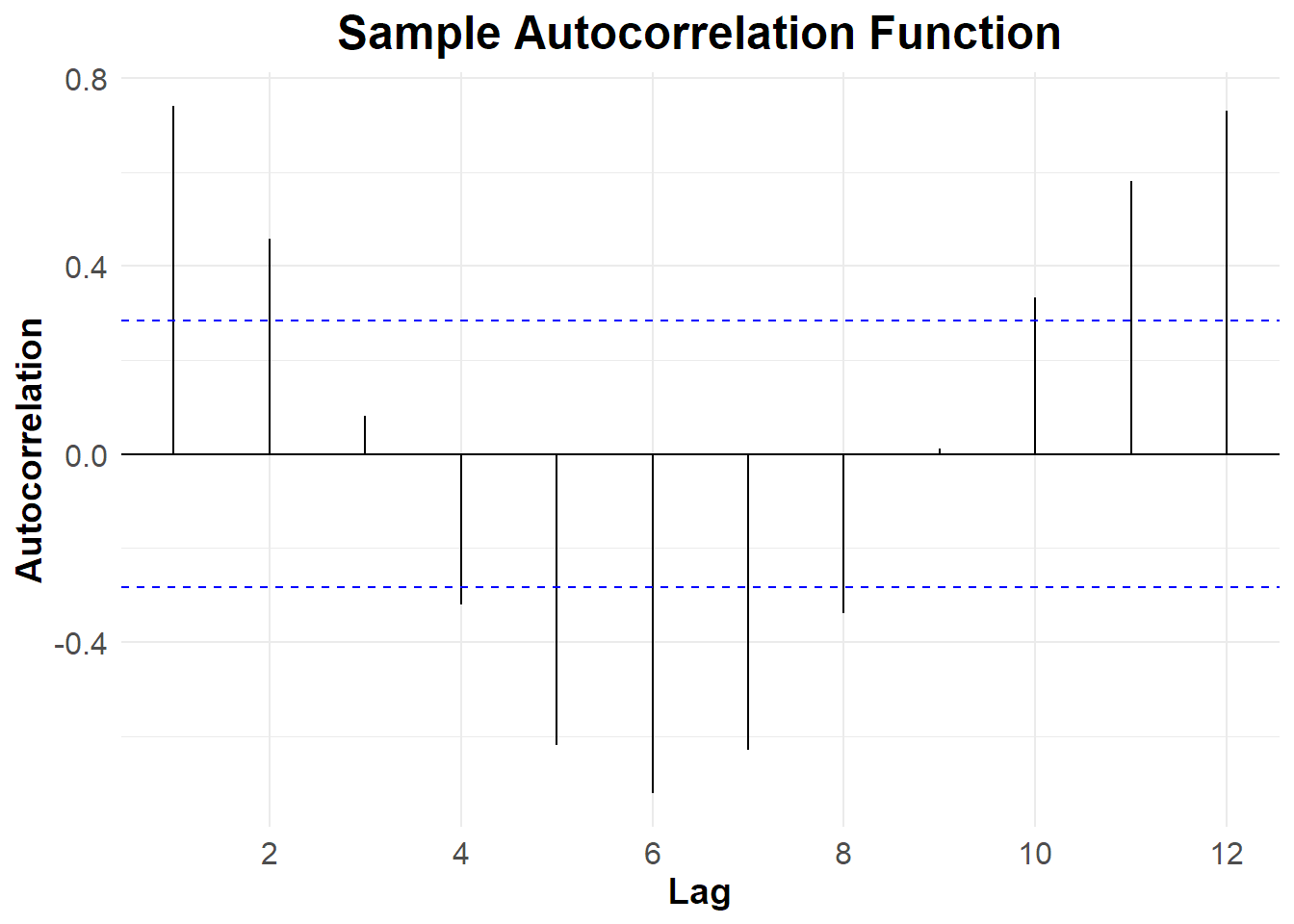
5.2判断该序列的平稳性和纯随机性
# 单位根检验library(tseries)
adf.test(ts_d5)
## Warning in adf.test(ts_d5): p-value smaller than printed p-value##
## Augmented Dickey-Fuller Test
##
## data: ts_d5
## Dickey-Fuller = -6.1123, Lag order = 3, p-value = 0.01
## alternative hypothesis: stationary# Ljung-Box检验
Box.test(ts_d5, lag = 12, type = "Ljung-Box")##
## Box-Ljung test
##
## data: ts_d5
## X-squared = 190.4, df = 12, p-value < 2.2e-16如果单位根检验的 p 值小于 0.05,则时间序列不是平稳的。如果 Ljung-Box 检验的 p 值小于 0.05,则时间序列不是纯随机的。根据结果,我们可以得出结论:该时间序列是非平稳的且非纯随机的。
6.1969年1月至1973年9月芝加哥海德公园内每28天发生的抢包案件数
6.1判断序列 的平稳性和纯随机性
d6 <- c(t(read.table('./时间序列分析——基于R(第2版)习题数据/习题2.6数据.txt', sep = '\t')));d6## [1] 10 15 10 10 12 10 7 7 10 14 8 17 14 18 3 9 11 10 6 12 14 10 25 29 33
## [26] 33 12 19 16 19 19 12 34 15 36 29 26 21 17 19 13 20 24 12 6 14 6 12 9 11
## [51] 17 12 8 14 14 12 5 8 10 3 16 8 8 7 12 6 10 8 10 5 NA NA# 设置主题
theme_custom <- function(base_size = 10, base_family = "myFont") {
theme(
text = element_text(size = base_size, family = base_family),
plot.title = element_text(hjust = 0.5, size = base_size*1.2, face = "bold", colour = '#004a7c'),
plot.subtitle = element_text(hjust = 0.5, size = base_size, face = "italic"),
axis.title = element_text(size = base_size*1.1, face = "bold", colour = '#1b262c'),
axis.text = element_text(size = base_size, colour = '#0f4c75'),
legend.title = element_text(size = base_size*1.1, face = "bold", colour = '#3282b8'),
legend.text = element_text(size = base_size, colour = '#bbe1fa')
)
}
# 画时序图library(ggplot2)
ggplot(data.frame(x = na.omit(d6), t = 1:length(na.omit(d6))), aes(x = t, y = x)) +
geom_line(color = "#3B4F63") +
labs(title = "Robberies in Heide Park (1969-1973)",
subtitle = "Recorded every 28 days",
x = "Time", y = "Number of robberies") +
theme_custom()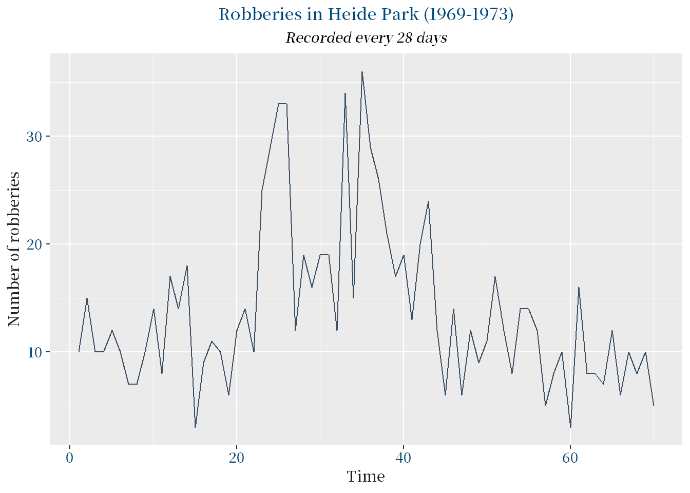
# 检验平稳性和纯随机性library(tseries)
adf.test(na.omit(d6)) # ADF检验
##
## Augmented Dickey-Fuller Test
##
## data: na.omit(d6)
## Dickey-Fuller = -2.168, Lag order = 4, p-value = 0.5069
## alternative hypothesis: stationarykpss.test(na.omit(d6)) # KPSS检验##
## KPSS Test for Level Stationarity
##
## data: na.omit(d6)
## KPSS Level = 0.35581, Truncation lag parameter = 3, p-value = 0.0962ggAcf(na.omit(d6))+
ggtitle("Autocorrelation of Robberies in Heide Park (1969-1973)")+
theme_custom()
ggPacf(na.omit(d6))+
  ggtitle("Partial Autocorrelation of Robberies in Heide Park (1969-1973)")+
  theme_custom()
print(adf.test(na.omit(d6)))##
## Augmented Dickey-Fuller Test
##
## data: na.omit(d6)
## Dickey-Fuller = -2.168, Lag order = 4, p-value = 0.5069
## alternative hypothesis: stationaryprint(kpss.test(na.omit(d6)))##
## KPSS Test for Level Stationarity
##
## data: na.omit(d6)
## KPSS Level = 0.35581, Truncation lag parameter = 3, p-value = 0.0962由ADF和KPSS检验的结果可以看出,序列${x_t}$和${y_t}$均不平稳。由ACF和PACF图可以看出,序列${x_t}$和${y_t}$均存在较强的自相关性和季节性。
6.2对序列进行函数运算: ,并判断序列
 的平稳性和纯随机性
# 计算差分序列
diff_data <- diff(na.omit(d6));diff_data
## [1] 5 -5 0 2 -2 -3 0 3 4 -6 9 -3 4 -15 6 2 -1 -4 6
## [20] 2 -4 15 4 4 0 -21 7 -3 3 0 -7 22 -19 21 -7 -3 -5 -4
## [39] 2 -6 7 4 -12 -6 8 -8 6 -3 2 6 -5 -4 6 0 -2 -7 3
## [58] 2 -7 13 -8 0 -1 5 -6 4 -2 2 -5# 画差分序列时序图
ggplot(data.frame(y = diff_data, t = 2:length(na.omit(d6))), aes(x = t, y = y)) +
geom_line(color = "#F15A60") +
labs(title = "Differenced Robberies in Heide Park (1969-1973)",
subtitle = "Recorded every 28 days",
x = "Time", y = "Difference in number of robberies") +
theme_custom()
# 检验平稳性和纯随机性
adf.test(diff_data) # ADF检验
## Warning in adf.test(diff_data): p-value smaller than printed p-value##
## Augmented Dickey-Fuller Test
##
## data: diff_data
## Dickey-Fuller = -4.3625, Lag order = 4, p-value = 0.01
## alternative hypothesis: stationarykpss.test(diff_data) # KPSS检验## Warning in kpss.test(diff_data): p-value greater than printed p-value##
## KPSS Test for Level Stationarity
##
## data: diff_data
## KPSS Level = 0.07078, Truncation lag parameter = 3, p-value = 0.1ggAcf(diff_data)+
ggtitle("Autocorrelation of Differenced Robberies in Heide Park (1969-1973)")+
theme_custom()
ggPacf(diff_data)+
  ggtitle("Partial Autocorrelation of Differenced Robberies in Heide Park (1969-1973)")+
  theme_custom()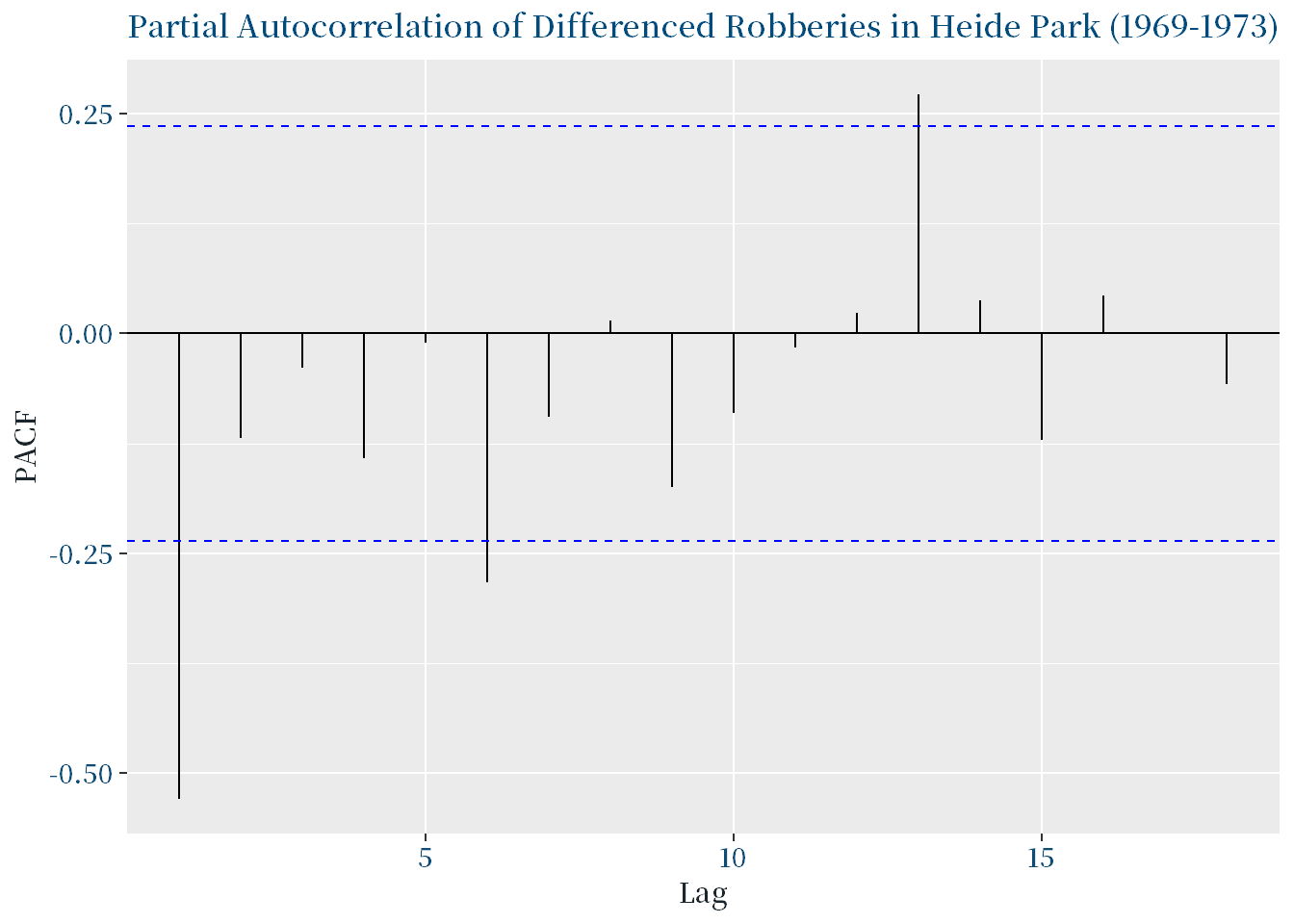
print(adf.test(diff_data))## Warning in adf.test(diff_data): p-value smaller than printed p-value##
## Augmented Dickey-Fuller Test
##
## data: diff_data
## Dickey-Fuller = -4.3625, Lag order = 4, p-value = 0.01
## alternative hypothesis: stationaryprint(kpss.test(diff_data))## Warning in kpss.test(diff_data): p-value greater than printed p-value##
## KPSS Test for Level Stationarity
##
## data: diff_data
## KPSS Level = 0.07078, Truncation lag parameter = 3, p-value = 0.1对于差分序列${y_t}$,其平稳性得到了明显改善。ADF和KPSS检验的结果均表明,差分序列${y_t}$是平稳的。同时,由ACF和PACF图可以看出,差分序列${y_t}$不存在明显的自相关性和季节性。
7.1915-2004年澳大利亚每年与枪支有关的凶杀案死亡率(每10万人)
7.1绘制时序图,考察平稳特征
d7 <- read.table('./时间序列分析——基于R(第2版)习题数据/习题2.7数据.txt', header = TRUE)
ts_d7 <- ts(d7$死亡率,start = c(1915));ts_d7
## Time Series:
## Start = 1915
## End = 2004
## Frequency = 1
## [1] 0.5215052 0.4248284 0.4250311 0.4771938 0.8280212 0.6156186 0.3666270
## [8] 0.4308883 0.2810287 0.4646245 0.2693951 0.5779049 0.5661151 0.5077584
## [15] 0.7507175 0.6808395 0.7661091 0.4561473 0.4977496 0.4193273 0.6095514
## [22] 0.4573370 0.5705478 0.3478996 0.3874993 0.5824285 0.2391033 0.2367445
## [29] 0.2626158 0.4240934 0.3652750 0.3750758 0.4090056 0.3891676 0.2402610
## [36] 0.1589496 0.4393373 0.5094681 0.3743465 0.4339828 0.4130557 0.3288928
## [43] 0.5186648 0.5486504 0.5469111 0.4963494 0.5308929 0.5957761 0.5570584
## [50] 0.5731325 0.5005416 0.5431269 0.5593657 0.6911693 0.4403485 0.5676662
## [57] 0.5969114 0.4735537 0.5923935 0.5975556 0.6334127 0.6057115 0.7046107
## [64] 0.4805263 0.7026860 0.7009017 0.6030854 0.6980919 0.5976560 0.8023421
## [71] 0.6017109 0.5993127 0.6025625 0.7016625 0.4995714 0.4980918 0.4975690
## [78] 0.6001830 0.3339542 0.2744370 0.3209428 0.5406671 0.4050209 0.2885961
## [85] 0.3275942 0.3132606 0.2575562 0.2138386 0.1861856 0.1592713autoplot(ts_d7, xlab = "年份", ylab = "死亡率(每10万人)")+
theme_custom()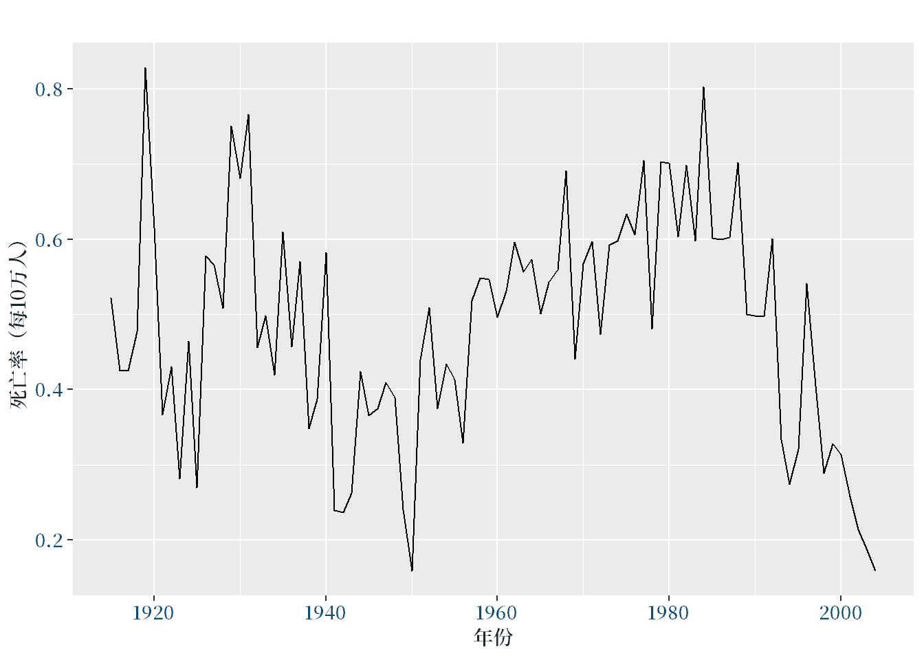
根据时序图可以看出,该序列的方差似乎并没有随着时间变化而发生显著的变化,因此可以初步认为该序列是平稳的。但是,为了进一步确定该序列的平稳性,需要绘制自相关图。
7.2绘制自相关图,分析该序列的平稳性
# 绘制自相关图
ggAcf(ts_d7, lag.max = 20)+
  ggtitle("自相关图")+
  theme_custom()
由自相关图可以看出,该序列存在显著的正自相关,且自相关系数衰减缓慢,这表明该序列不是平稳的。为了进一步确定该序列的平稳性,需要对其进行一阶差分,得到一阶差分后的序列并绘制时序图和自相关图。
7.3如果该序列是平稳序列,则分析该序列的纯随机性,如果是非平稳序列,则分析该序列一阶差分后序列的平稳性。
# 进行一阶差分
diff_ts_d7 <- diff(ts_d7)
par(mfrow=c(1,2))
# 绘制差分后的时序图
autoplot(diff_ts_d7, xlab = "年份", ylab = "死亡率(每10万人)")+
  theme_custom()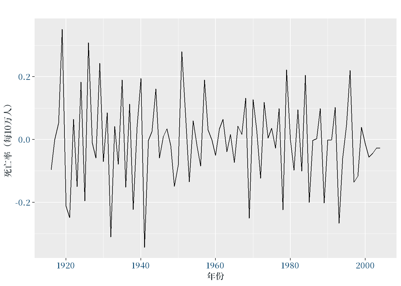
# 绘制差分后的自相关图
ggAcf(diff_ts_d7, lag.max = 20)+
  ggtitle("一阶差分后的自相关图")+
  theme_custom()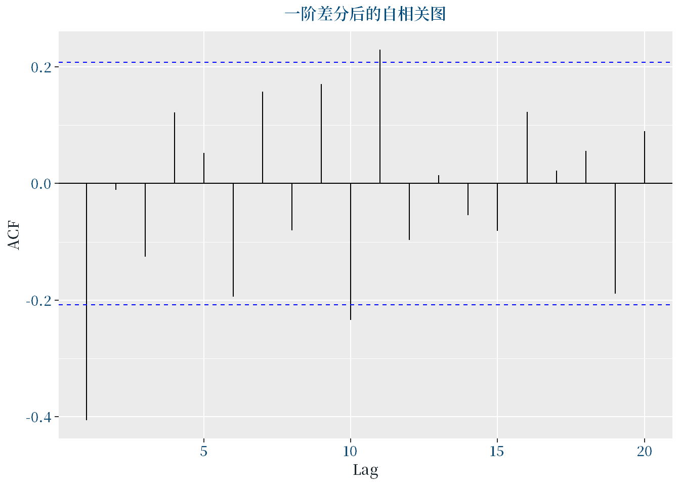
由于差分后序列的自相关图中,几乎所有的自相关系数都在显著水平之下,表明序列具有平稳性,因此可以进行纯随机性检验。
library(lawstat)##
## 载入程辑包:'lawstat'## The following object is masked from 'package:tseries':
##
## runs.testruns.test(diff_ts_d7)##
## Runs Test - Two sided
##
## data: diff_ts_d7
## Standardized Runs Statistic = 2.4535, p-value = 0.01415由于p值大于0.05,无法拒绝原假设,因此认为该序列是一个纯随机序列。

8.1860-1955年密歇根湖每月平均水位的最高值序列
8.1绘制时序图,考察平稳特征
d8 <- read.table('./时间序列分析——基于R(第2版)习题数据/习题2.8数据.txt', header = TRUE)
ts_d8 <- ts(d8$水位,start = c(1860));ts_d8
## Time Series:
## Start = 1860
## End = 1955
## Frequency = 1
## [1] 83.30 83.50 83.20 82.60 82.20 82.10 81.70 82.20 81.60 82.10 82.70 82.80
## [13] 81.50 82.20 82.30 82.10 83.60 82.70 82.50 81.50 82.10 82.20 82.60 83.30
## [25] 83.10 83.30 83.70 82.90 82.30 81.80 81.60 80.90 81.00 81.30 81.40 80.20
## [37] 80.00 80.85 80.83 81.10 80.70 81.10 80.83 80.82 81.50 81.60 81.50 81.60
## [49] 81.80 81.10 80.50 80.00 80.70 81.30 80.70 80.00 81.10 81.87 81.91 81.30
## [61] 81.00 80.50 80.60 79.80 79.60 78.49 78.49 79.60 80.60 82.30 81.20 79.10
## [73] 78.60 78.70 78.00 78.60 78.70 78.60 79.70 80.00 79.30 79.00 80.20 81.50
## [85] 80.80 81.00 80.96 81.10 80.80 79.70 80.00 81.60 82.70 82.10 81.70 81.50# 绘制时序图library(ggplot2)
ggplot(d8, aes(x = 年, y = 水位)) +
geom_line(color = "steelblue", size = 1) +
labs(title = "密歇根湖水位(1860-1955)", x = "年", y = "水位") +
theme_custom()
根据时序图可以看出,该序列存在周期性波动,但整体趋势基本稳定。
8.2绘制自相关图,分析该序列的平稳性
# 绘制自相关图
ggAcf(ts_d8, lag.max = 30)+
  ggtitle("自相关图") +
  xlab("Lag") +
  ylab("ACF") +
  theme_custom()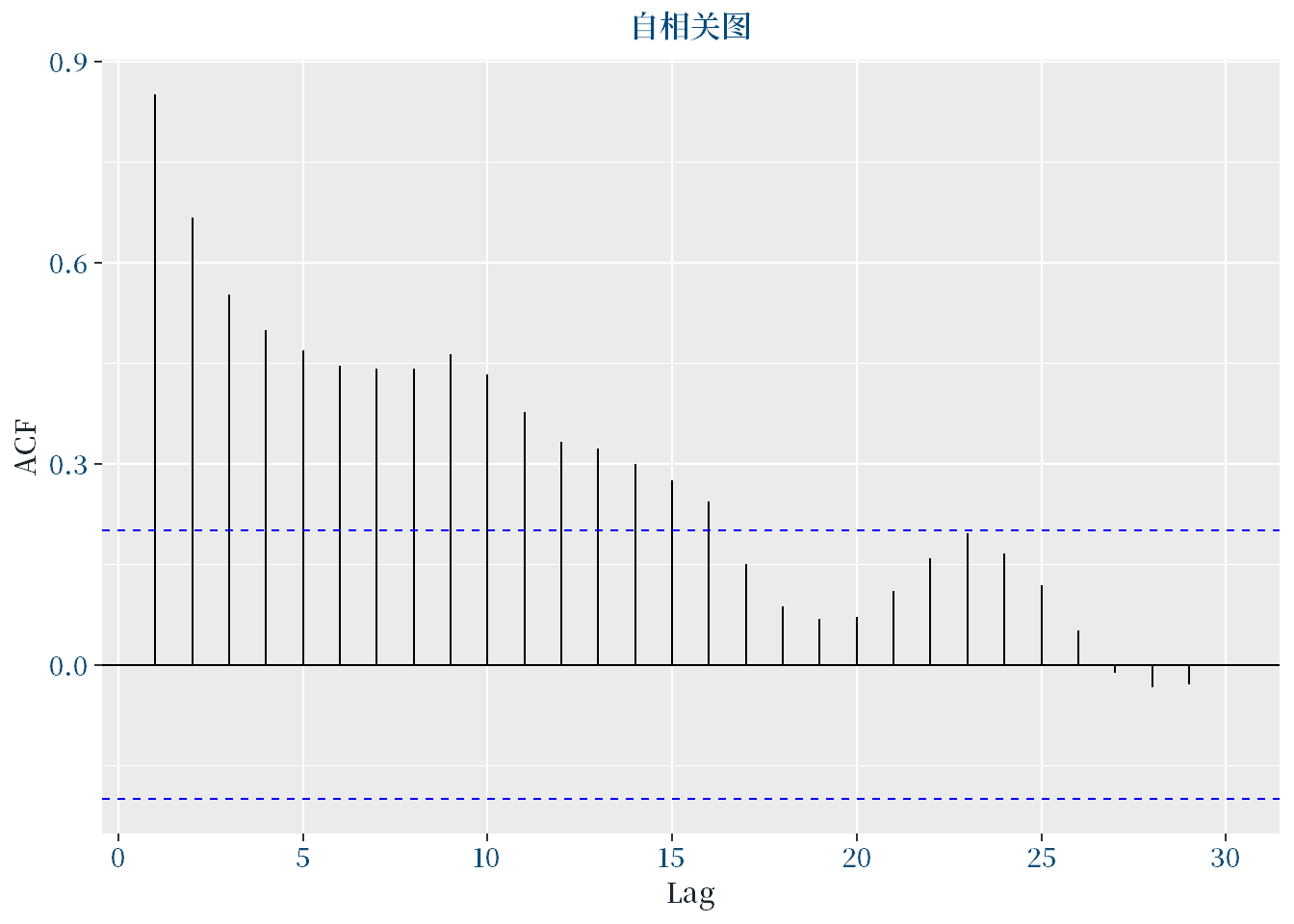
自相关图显示出较强的正自相关性,表明该序列不是平稳序列,需要进行差分。
8.3如果该序列是平稳序列,则分析该序列的纯随机性,如果是非平稳序列,则分析该序列一阶差分后序列的平稳性。
# 进行一阶差分
diff_ts_d8 <- diff(ts_d8)
ggplot() +
geom_line(aes(x = d8$年[-1], y = diff_ts_d8), color = "steelblue", size = 1) +
labs(title = "密歇根湖水位一阶差分序列(1861-1955)", x = "年", y = "水位差分") +
theme_custom()## Don't know how to automatically pick scale for object of type <ts>. Defaulting
## to continuous.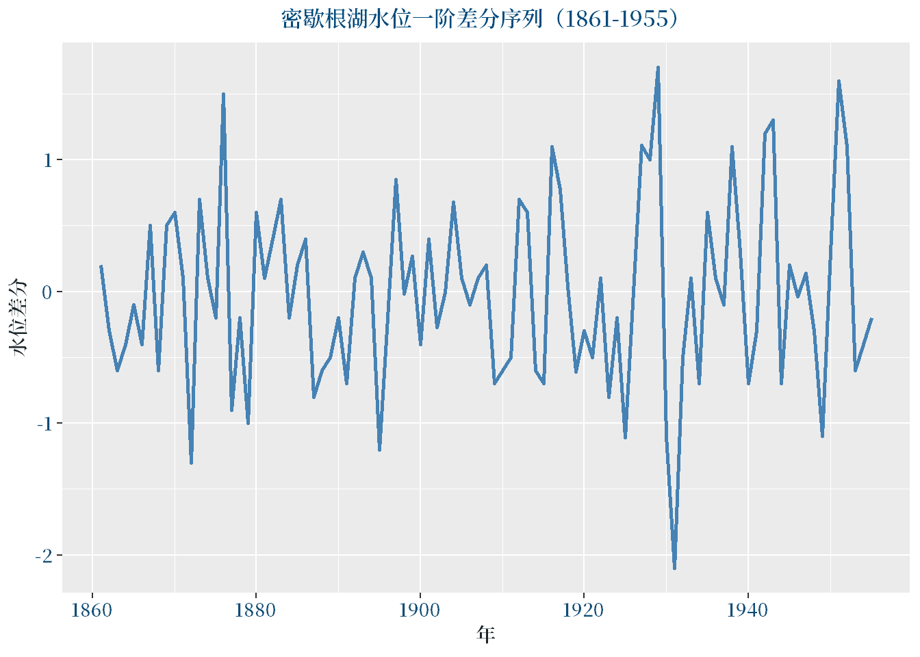
# 绘制自相关图
ggAcf(diff_ts_d8, lag.max = 30)+
  ggtitle("一阶差分自相关图")+
  theme_custom()
一阶差分的时序图显示出,一阶差分序列的波动已经变得更加平稳。自相关图显示出,一阶差分序列的自相关系数都在置信区间内,表明一阶差分序列已经平稳。
1.本文参考资料为时间序列分析——基于R/王燕编著. —5版. —北京:中国人民大学出版社,2020.6
(基于R应用的统计学丛书)
ISBN 978-7-300-27898-8
2.本文的部分代码参考了ChatGPT给出的方法,经检验后有效。