哈希函数的学习算法整理

前言

如果你对这篇文章感兴趣，可以点击「【访客必读 - 指引页】一文囊括主页内所有高质量博客」，查看完整博客分类与对应链接。

---

概述

哈希函数学习的两个步骤：

• 转为二进制编码：可以先降维成实数，再转为二进制，也可以直接学习一个二进制编码；
• 学习哈希映射函数：基于二进制编码设计或学习哈希方式，使得相似元素靠近，不相似元素远离。

根据哈希函数性质，可做如下分类：

• 数据无关的方法 (Data-Independent Methods)
  • 特点：哈希函数与训练集无关，通常为随机投影或手动构造
  • 举例：Locality-sensitive hashing (LSH), Shift invariant kernel hashing (SIKH), MinHash;
• 数据相关的方法 (Data-Dependent Methods)
  • 特点：哈希函数通过训练集学习得到
  • 分类：单模态哈希（无监督 / 有监督）、基于排序的方法（监督信息为排序序列）、多模态哈希、深度哈希

---

无监督哈希 (Unsupervised Hashing)

问题定义：

• 输入：特征向量 { x i } \{\mathbf{x}_i\} { xi​}，对应矩阵 $\mathbf{X}$；
• 输出：二进制编码 { b i } \{\mathbf{b}_i\} { bi​}，对应矩阵 $\mathbf{B}$，相似的特征对应相似的编码

PCA Hashing (PCAH)

选取矩阵 ${\mathbf{XX}}^{\top }$ 最大的 $m$ 个特征向量，组成投影矩阵 $\mathbf{W}\in {\mathbb{R}}^{d\times m}$，并定义哈希函数为：
$$h(\mathbf{x})=\mathrm{sgn}\left({\mathbf{W}}^{\top }\mathbf{x}\right).$$

Spectral Hashing (SH)

min ⁡ { y i }     ∑ i j W i j ∥ y i − y j ∥ 2  s.t.    y i ∈ { − 1 , 1 } k ∑ i y i = 0 1 n ∑ i y i y i ⊤ = I \begin{aligned} \mathop{\min}\limits_{\left\{\mathbf{y}_i\right\}} \ \ \ & \sum_{i j} W_{i j}\left\|\mathbf{y}_i-\mathbf{y}_j\right\|^2 \\ \text { s.t.} \ \ \ & \mathbf{y}_i \in\{-1,1\}^k \\ &\sum_i \mathbf{y}_i=0 \\ &\frac{1}{n} \sum_i \mathbf{y}_i \mathbf{y}_i^\top=\mathbf{I} \end{aligned} { yi​}min​    s.t.   ​ij∑​Wij​∥yi​−yj​∥2yi​∈{ −1,1}ki∑​yi​=0n1​i∑​yi​yi⊤​=I​

其中 $W_{ij}$ 为 ${\mathbf{x}}_i$ 和 ${\mathbf{x}}_j$ 的相似度，第二个约束意味着所有数据映射后，每一位上 $1$ 和 $-1$ 的数量相同，第三个约束意味着不同位之间没有关联。上述优化问题为整数规划，难以求解，可将 y i ∈ { − 1 , 1 } k \mathbf{y}_i \in\{-1,1\}^k yi​∈{ −1,1}k 约束取消，对问题进行放松，并将求得的 { y i } \{\mathbf{y}_i\} { yi​} 每一位通过 $\mathrm{sgn}$ 函数映射，得到最终的二进制编码。

Anchor Graph Hashing (AGH)

对 $\mathbf{X}$ 使用 k-means 聚类，得到 { u j ∈ R d } j = 1 m \{\mathbf{u}_j\in \mathbb{R}^d\}_{j=1}^m { uj​∈Rd}j=1m​，重新定义矩阵 $\mathbf{Z}\in {\mathbb{R}}^{n\times m}$：
$$Z_{ij}=\{\begin{array}{l}\frac{\exp \left(-{\mathcal{D}}^2\left({\mathbf{x}}_i,{\mathbf{u}}_j\right)/t\right)}{{\sum }_{j^{\prime }\in {\mathcal{J}}_i}\exp \left(-{\mathcal{D}}^2\left({\mathbf{x}}_i,{\mathbf{u}}_{j^{\prime }}\right)/t\right)},\forall j\in {\mathcal{J}}_i\\ 0,\text{ otherwise }\end{array}$$

其中 ${\mathcal{J}}_i$ 为一个下标集合，对应 { u j ∈ R d } j = 1 m \{\mathbf{u}_j\in \mathbb{R}^d\}_{j=1}^m { uj​∈Rd}j=1m​ 中 $s$ 个离 ${\mathbf{x}}_i$ 最近的点的下标。定义哈希函数为：
$$h(\mathbf{x})=\mathrm{sign}\left(W^{\top }z(\mathbf{x})\right),$$

其中 $W=\sqrt{n}{\Lambda }^{-1/2}V{\Sigma }^{-1/2}$，$\Lambda =\mathrm{diag}\left(Z^{\top }1\right)$，$V$ 和 $\Sigma$ 由矩阵 ${\Lambda }^{-1/2}{Z}^{\top }{\Lambda }^{-1/2}$ 的特征向量和特征值组成。该方法整体目标与 Spectral Hashing 一致，但通过引入 Anchor，使问题求解得到了加速，时间复杂度从 $O(n^3)$ 降至为 $O(n{m}^2)$。具体细节可参照原论文。

---

有监督哈希 (Supervised Hashing)

问题定义：

• 输入：特征向量 { x i } \{\mathbf{x}_i\} { xi​}，对应矩阵 $\mathbf{X}$，类别向量 { y i } \{\mathbf{y}_i\} { yi​}，对应矩阵 $\mathbf{Y}$
• 输出：二进制编码 { b i } \{\mathbf{b}_i\} { bi​}，对应矩阵 $\mathbf{B}$，相同类别对应相似编码

常见算法如下所示，具体信息见参考资料，此处不再展开。

---

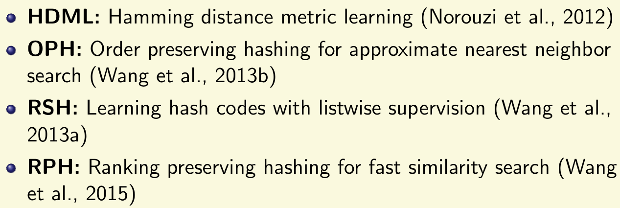
基于排序的方法 (Ranking-based Methods)

该部分属于有监督哈希一类，不过监督信息从标记变为了排序信息，例如三元组 $\left(x,x^{+},x^{-}\right)$。该部分涉及的常见算法如下：

---

参考资料

• Learning to Hash
• Learning to Hash for Big Data: A Tutorial