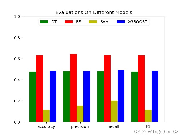
在之前的项目中,有关声纹识别和声源定位相关的实践较少,项目的原因,后续会陆续增加这块的投入,周末闲来无事就像先简单开发实践基础项目,这里主要是基于mfcc、csc、zcr几种特征提取方法集合决策树、支持向量机、随机森林和XGBoost几种模型来实现声纹识别,话不多说,首先看下效果:

简单看下数据集:
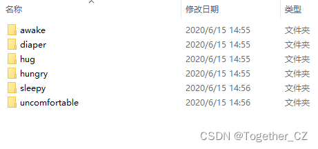
awake:
diaper:
hug:

hungry:
sleepy:
uncomfortable:
数据解析特征提取核心实现如下所示:
feature=[]
for one_label in os.listdir(dataDir):
    oneDir=dataDir+one_label+"/"
    for one_file in os.listdir(oneDir):
        print("one_file: ", one_file)
        try:
            one_path=oneDir+one_file
            data,RATE = librosa.load(one_path, 44100)
            f1=mfcc(data)
            f2=csc(data)
            f3=zcr(data)
            one_vec=np.hstack([f1, f2, f3]).tolist()
            one_vec.append(one_label)
            feature.append(one_vec)
        except Exception as e:
            print("Exception: ", e)
print("feature_length: ", len(feature))
with open(save_path,"w") as f:
    f.write(json.dumps(feature))
生成feature文件后,接下来初始化搭建模型,这里以RF为例如下:
with open(data) as f:
    data_list = json.load(f)
x_list = [one[:-1] for one in data_list]
y_list = [one[-1] for one in data_list]
print("y_list: ", list(set(y_list)))
X_train, X_test, y_train, y_test = splitData(x_list, y_list, ratio=rationum)
try:
    model = loadModel(model_path="rf.pkl")
except:
    model = RandomForestClassifier(n_estimators=100)
    model.fit(X_train, y_train)
y_pred = model.predict(X_test)
print("RF model accuracy: ", model.score(X_test, y_test))
# 指标计算
res_dict = {}
Precision, Recall, F1 = calThree(y_test, y_pred)
res_dict["precision"] = Precision
res_dict["recall"] = Recall
res_dict["F1"] = F1
res_dict["accuracy"] = F1
print("res_dict: ", res_dict)
saveModel(model, save_path=model_path)
return res_dict
结果如下:
============================Loading classifyModel============================
y_list:  ['hug', 'diaper', 'hungry', 'uncomfortable', 'awake', 'sleepy']
=================splitData shape============================
688 688
230 230
DT model accuracy:  0.48695652173913045
F1:  0.47760615805170265
Precision:  0.47929344540393237
Recall:  0.479810176927286
res_dict:  {'precision': 0.47929344540393237, 'recall': 0.479810176927286, 'F1': 0.47760615805170265, 'accuracy': 0.47760615805170265}
y_list:  ['hug', 'diaper', 'hungry', 'uncomfortable', 'awake', 'sleepy']
=================splitData shape============================
688 688
230 230
RF model accuracy:  0.6434782608695652
F1:  0.6319053593191524
Precision:  0.6449388328420587
Recall:  0.6348164749454582
res_dict:  {'precision': 0.6449388328420587, 'recall': 0.6348164749454582, 'F1': 0.6319053593191524, 'accuracy': 0.6319053593191524}
y_list:  ['hug', 'diaper', 'hungry', 'uncomfortable', 'awake', 'sleepy']
=================splitData shape============================
688 688
230 230
SVM model accuracy:  0.2217391304347826
F1:  0.11388339920948616
Precision:  0.15566037735849056
Recall:  0.20020325203252032
res_dict:  {'precision': 0.15566037735849056, 'recall': 0.20020325203252032, 'F1': 0.11388339920948616, 'accuracy': 0.11388339920948616}
y_list:  ['hug', 'diaper', 'hungry', 'uncomfortable', 'awake', 'sleepy']
=================splitData shape============================
688 688
230 230
XGBOOST model accuracy:  0.5
F1:  0.48469331276155714
Precision:  0.48176557040929696
Recall:  0.49042707402902413
res_dict:  {'precision': 0.48176557040929696, 'recall': 0.49042707402902413, 'F1': 0.48469331276155714, 'accuracy': 0.48469331276155714}
四种模型对比结果如下:
{
    "DT": {
        "precision": 0.47929344540393239,
        "recall": 0.479810176927286,
        "F1": 0.47760615805170267,
        "accuracy": 0.47760615805170267
    },
    "RF": {
        "precision": 0.6449388328420587,
        "recall": 0.6348164749454582,
        "F1": 0.6319053593191524,
        "accuracy": 0.6319053593191524
    },
    "SVM": {
        "precision": 0.15566037735849057,
        "recall": 0.20020325203252033,
        "F1": 0.11388339920948616,
        "accuracy": 0.11388339920948616
    },
    "XGBOOST": {
        "precision": 0.48176557040929698,
        "recall": 0.49042707402902416,
        "F1": 0.48469331276155716,
        "accuracy": 0.48469331276155716
    }
}
为了直观对比这里对其进行可视化展示,如下所示: