目录
本项目根据Working with Spatio-temporal data in Python进行翻译整理,译者:lqy,华东师范大学大气科学专业
数据上传至和鲸社区数据集 | Python气象时空数据处理(演示数据)
获得代码运行环境,一键运行项目请点击>>快速入门基于Python的时空数据分析快速入门基于Python的时空数据分析
一、时空数据的常见格式
空间数据以许多不同的方式表示,并以不同的文件格式存储。本项目将重点介绍两种类型的空间数据:栅格数据和矢量数据。
1. 常见格式的简介
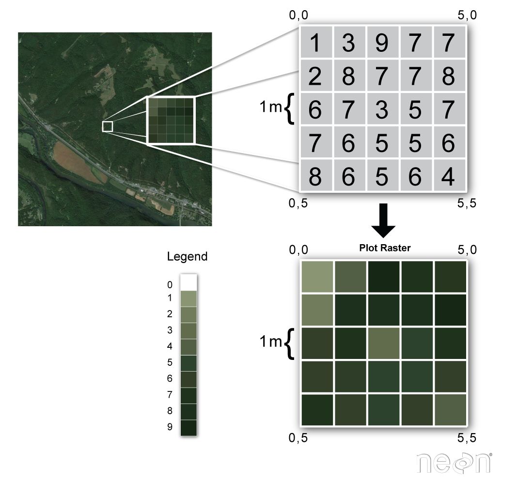
栅格数据 :保存在统一格网中,并在地图上以像素的形式呈现。每个像素都包含一个表示地球表面上某个区域的值。
栅格常见格式:netCDF、TIF
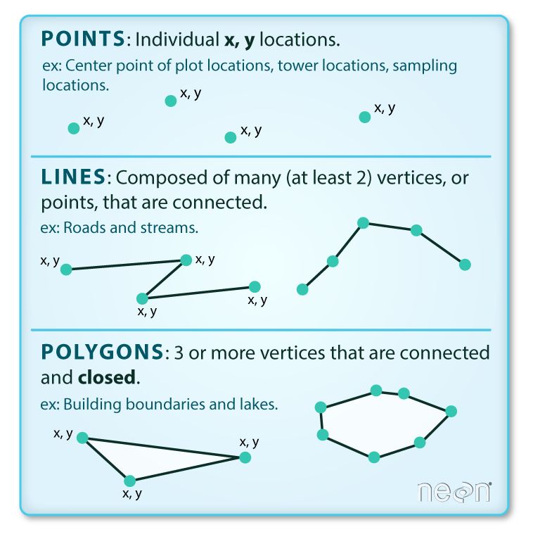
矢量数据:通常用于存储道路和地块位置、州、国家和湖泊边界等内容。由离散的几何位置(x,y 值)组成,这些位置称为顶点,用于定义空间对象的形状。
矢量常见格式:shapefile、geojson
-
点:每个单独的点由单个 x、y 坐标定义。矢量点文件中可以有许多点。点数据的示例包括:采样位置、单个树的位置或地块的位置。
-
线:线由许多(至少 2 个)连接的折点组成。例如,道路或溪流可以用一条线表示。这条线由一系列线段组成,道路或溪流中的每个"弯道"都表示一个已定义 x、y 位置的顶点。
-
多边形:多边形由 3 个或更多连接且"封闭"的顶点组成。通常由多边形表示的对象包括:绘图边界、湖泊、海洋以及州或国家边界的轮廓。
使用 shapefile 时,请务必记住,shapefile 由 3 个(或更多)文件组成:
-
.shp:包含所有要素的几何的文件。
-
.shx:为几何图形编制索引的文件。
-
.dbf:以表格格式存储要素属性的文件。
这些文件需要具有相同的名称并存储在同一目录(文件夹)中,才能在GIS,R或Python工具中正确打开。
有时,形状文件将具有其他关联的文件,包括:
-
.prj:包含投影格式信息的文件,包括坐标系和投影信息。它是一个使用已知文本 (WKT) 格式描述投影的纯文本文件。
-
.sbn 和 .sbx:作为要素的空间索引的文件。
-
.shp.xml:作为 XML 格式的地理空间元数据的文件(例如.ISO 19115 或 XML 格式)。
2. 常见格式的读取
导入模块
from netCDF4 import Dataset
import netCDF4 as nc
import matplotlib.pyplot as plt
from osgeo import gdal, ogr
from mpl_toolkits.basemap import Basemap
读取nc数据
f = nc.Dataset('/home/mw/input/metos8969/metos/MISR_AM1_CGLS_MAY_2007_F04_0031.hdf','r')
print("Metadata for the dataset:")
print(f)
print("List of available variables (or key): ")
f.variables.keys()
print("Metadata for 'NDVI average' variable: ")
f.variables["NDVI average"]
f.close()
创建nc数据
# 创建nc文件及维度
f = nc.Dataset('orography.nc', 'w')
f.createDimension('time', None)
f.createDimension('z', 3)
f.createDimension('y', 4)
f.createDimension('x', 5)
lats = f.createVariable('lat', float, ('y', ), zlib=True)
lons = f.createVariable('lon', float, ('x', ), zlib=True)
orography = f.createVariable('orog', float, ('y', 'x'), zlib=True, least_significant_digit=1, fill_value=0)
# 创建一维数组
lat_out  = [60, 65, 70, 75]
lon_out  = [ 30,  60,  90, 120, 150]
# 创建二维数组
data_out = np.arange(4*5)
data_out.shape = (4,5)
orography[:] = data_out
lats[:] = lat_out
lons[:] = lon_out
# 关闭文件
f.close()


# 打开创建后的nc数据
f = nc.Dataset('orography.nc', 'r')
print(f)
f.close()


# 输出nc文件的数值
f = nc.Dataset('orography.nc', 'r')
lats = f.variables['lat']
lons = f.variables['lon']
orography = f.variables['orog']
print(lats[:])
print(lons[:])
print(orography[:])
f.close()


# nc文件的数值的切片打印
f = nc.Dataset('orography.nc', 'r')
lats = f.variables['lat']
lons = f.variables['lon']
orography = f.variables['orog']
print(lats[:])
print(lons[:])
print(orography[:][3,2])
f.close()
绘制nc数据
f = nc.Dataset('/home/mw/input/metos8969/metos/MISR_AM1_CGLS_MAY_2007_F04_0031.hdf','r')
data = f.variables['NDVI average'][:]
print(type(data))
print(data.shape)
plt.imshow(data)
plt.show()
f.close()
f = nc.Dataset('/home/mw/input/metos8969/metos/OMI-Aura_L3-OMTO3e_2017m0105_v003-2017m0203t091906.he5')
data = f.groups['HDFEOS'].groups['GRIDS'].groups['OMI Column Amount O3'].groups['Data Fields'].variables['ColumnAmountO3']
plt.imshow(data)
plt.show()
f.close()
f = nc.Dataset('/home/mw/input/metos8969/metos/AIRS.2002.08.30.227.L2.RetStd_H.v6.0.12.0.G14101125810.hdf')
data = f.variables['topog']
plt.imshow(data)
plt.show()
f.close()
读取GeoTIFF数据
datafile = gdal.Open('/home/mw/input/metos8969/metos/Southern_Norway_and_Sweden.2017229.terra.1km.tif')
print( "Driver: ",datafile.GetDriver().ShortName, datafile.GetDriver().LongName)
print( "Size is ", datafile.RasterXSize, datafile.RasterYSize)
print( "Bands = ", datafile.RasterCount)
print( "Coordinate System is:", datafile.GetProjectionRef ())
print( "GetGeoTransform() = ", datafile.GetGeoTransform ())
print( "GetMetadata() = ", datafile.GetMetadata ())
绘制GeoTIFF数据
# 分别读取3个波段
bnd1 = datafile.GetRasterBand(1).ReadAsArray()
bnd2 = datafile.GetRasterBand(2).ReadAsArray()
bnd3 = datafile.GetRasterBand(3).ReadAsArray()
# 显示单波段影像
plt.imshow(bnd1)
plt.show()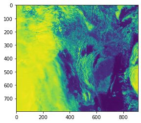
# RGB通道合成真彩色图像
print(type(bnd1), bnd1.shape)
print(type(bnd2), bnd3.shape)
print(type(bnd3), bnd3.shape)
img = np.dstack((bnd1,bnd2,bnd3))
print(type(img), img.shape)
plt.imshow(img)
plt.show()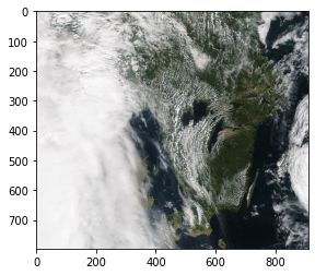
读取Shapefile数据
shapedata = ogr.Open('/home/mw/input/metos8969/metos/Norway_places')
layer = shapedata.GetLayer()
places_norway = []
for i in range(layer.GetFeatureCount()):
    feature = layer.GetFeature(i)
    name = feature.GetField("NAME")
    geometry = feature.GetGeometryRef()
    places_norway.append([i,name,geometry.GetGeometryName(), geometry.Centroid().ExportToWkt()])

print(places_norway[0:10])
绘制Shapefile数据
fig = plt.figure(figsize=[12,15])  # a new figure window
ax = fig.add_subplot(1, 1, 1)  # specify (nrows, ncols, axnum)
ax.set_title('Cities in Norway', fontsize=14)

map = Basemap(llcrnrlon=-1.0,urcrnrlon=40.,llcrnrlat=55.,urcrnrlat=75.,
             resolution='i', projection='lcc', lat_1=65., lon_0=5.)

map.drawmapboundary(fill_color='aqua')
map.fillcontinents(color='#ffe2ab',lake_color='aqua')
map.drawcoastlines()

shapedata = ogr.Open('/home/mw/input/metos8969/metos/Norway_places')
layer = shapedata.GetLayer()
for i in range(layer.GetFeatureCount()):
    feature = layer.GetFeature(i)
    name = feature.GetField("NAME")
    type = feature.GetField("TYPE")
    if type == 'city':
        geometry = feature.GetGeometryRef()
        lon = geometry.GetPoint()[0]
        lat = geometry.GetPoint()[1]
        x,y = map(lon,lat)
        map.plot(x, y, marker='o', color='red', markersize=8, markeredgewidth=2)
        ax.annotate(name, (x, y), color='blue', fontsize=14)

plt.show()
fig = plt.figure(figsize=[12,15])  # a new figure window
ax = fig.add_subplot(1, 1, 1)  # specify (nrows, ncols, axnum)

map = Basemap(llcrnrlon=-1.0,urcrnrlon=40.,llcrnrlat=55.,urcrnrlat=75.,
             resolution='i', projection='lcc', lat_1=65., lon_0=5.)
map.drawmapboundary(fill_color='aqua')
map.fillcontinents(color='#ffe2ab',lake_color='aqua')
map.drawcoastlines()
norway_roads= map.readshapefile('/home/mw/input/metos8969/metos/Norway_roads/roads', 'roads')

plt.show()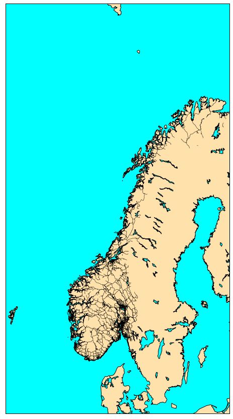
la = ogr.Open('/home/mw/input/metos8969/metos/la_city.geojson')
nblayer = la.GetLayerCount()
print("Number of layers: ", nblayer)
layer = la.GetLayer()
cities_us = []
for i in range(layer.GetFeatureCount()):
    feature = layer.GetFeature(i)
    name = feature.GetField("NAME")
    geometry = feature.GetGeometryRef()
    cities_us.append([i,name,geometry.GetGeometryName(), geometry.GetPoints()])

print(cities_us)
shapedata = ogr.Open('/home/mw/input/metos8969/metos/no-all-all.geojson')
nblayer = shapedata.GetLayerCount()
print("Number of layers: ", nblayer)
layer = shapedata.GetLayer()
county_norway = []
for i in range(layer.GetFeatureCount()):
feature = layer.GetFeature(i)
name = feature.GetField("NAVN")
geometry = feature.GetGeometryRef()
county_norway.append([i,name,geometry.GetGeometryName(), geometry.Centroid().GetPoint()])
print(county_norway[0:10])二、时空数据的可视化
导入模块
import matplotlib.pyplot as plt
import matplotlib.dates
import numpy as np
import pandas as pd
import datetime
import netCDF4 as nc
from matplotlib import colors as c
from mpl_toolkits.basemap import Basemap, shiftgrid
from mpl_toolkits.axes_grid1.inset_locator import zoomed_inset_axes
from mpl_toolkits.axes_grid1.inset_locator import mark_inset
import numpy.ma as ma
from osgeo import gdal, ogr
from matplotlib.patches import Polygon
from matplotlib.collections import PatchCollection
from matplotlib.patches import PathPatch
1D数据绘制
fig = plt.figure()  # 新窗口
ax = fig.add_subplot(1, 1, 1)  # 添加子图
fig = plt.figure()  # 新窗口
ax = fig.add_subplot(1, 1, 1)  # 添加子图
ax.set_title('Title of my subplot', fontsize=14)
# x轴标签
ax.set_xticklabels(np.arange(10), rotation=45, fontsize=10 )
# x轴标题
ax.set_xlabel("title for x-axis")
# x轴刻度
ax.set_xticks(np.arange(0, 10, 1.0))
# y轴标签
ax.set_yticklabels(np.arange(5), rotation=45, fontsize=10 )
# y轴标题
ax.set_ylabel("title for y-axis")
# y轴刻度
ax.set_yticks(np.arange(0, 5, 1.0))
plt.show()
dates = [datetime.date( 2001,6,1),
     datetime.date( 2001,6,2),
     datetime.date( 2001,6,3),
     datetime.date( 2001,6,4),
     datetime.date( 2001,6,5),
     datetime.date( 2001,6,6),
     datetime.date( 2001,6,7),
     datetime.date( 2001,6,8),
     datetime.date( 2001,6,9),
     datetime.date( 2001,6,10)]
# NAO 指数
nao_index = [ 0.132, -0.058, -0.321, -0.395, -0.216, -0.082, -0.023, -0.012, -0.012, -0.02]


fig = plt.figure()  # 新窗口
ax = fig.add_subplot(1, 1, 1)  # 添加子图
# 设置标题
ax.set_title('Time series for NAO index', fontsize=14)
# 设置x轴标签
ax.set_xticks(dates)
# 设置x轴刻度
ax.set_xticklabels(dates, rotation=45, fontsize=10)
# 设置x轴标题
ax.set_xlabel("Dates (YYYY-MM-DD)")
# 设置y轴标题
ax.set_ylabel("NAO index")
# 绘制NAO指数
ax.plot(dates, nao_index)
plt.show()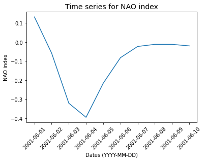
fig = plt.figure()  # 新窗口
ax = fig.add_subplot(1, 1, 1)  # 添加子图
# 设置标题
ax.set_title('Time series for NAO index', fontsize=14)
# 设置x轴标签
ax.set_xticks(dates)
# 设置x轴刻度
ax.set_xticklabels(dates, rotation=45, fontsize=10)
# 设置x轴标题
ax.set_xlabel("Dates")
# 设置y轴标题
ax.set_ylabel("NAO index")
# 设置日期格式
ax.xaxis.set_major_formatter(matplotlib.dates.DateFormatter('%a %d %b %Y'))
# 绘制NAO指数
ax.plot(dates, nao_index, 'r.-')
plt.show()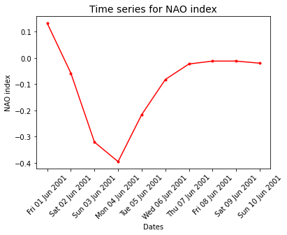
2D数据绘制
f = nc.Dataset("/home/mw/input/metos8969/metos/EI_VO_850hPa_Summer2001.nc", "r")
print(f)
f.close()

# 读取涡度变量
f = nc.Dataset('/home/mw/input/metos8969/metos/EI_VO_850hPa_Summer2001.nc', 'r')
lats = f.variables['lat'][:]
lons = f.variables['lon'][:]
VO = f.variables['VO'][0,0,:,:]*100000
fig = plt.figure(figsize=[12,15])  # 新窗口
ax = fig.add_subplot(1, 1, 1)  # 添加子图
ax.set_title('ECMWF ERA-Interim VO at 850 hPa 2001-06-01 00:00', fontsize=14)

map = Basemap(projection='cyl',llcrnrlat=-90,urcrnrlat=90, llcrnrlon=-180,urcrnrlon=180,resolution='c', ax=ax)
map.drawcoastlines()
map.fillcontinents(color='#ffe2ab')
# 添加经纬度
map.drawparallels(np.arange(-90.,120.,30.),labels=[1,0,0,0])
map.drawmeridians(np.arange(-180.,180.,60.),labels=[0,0,0,1])

# 经度范围设置为[-180,180]
VO, lons = shiftgrid(180.,VO,lons,start=False)
llons, llats = np.meshgrid(lons, lats)
x,y = map(llons,llats)
# 设置色阶
cmap = c.ListedColormap(['#00004c','#000080','#0000b3','#0000e6','#0026ff','#004cff',
                         '#0073ff','#0099ff','#00c0ff','#00d900','#33f3ff','#73ffff','#c0ffff',
                         (0,0,0,0),
                         '#ffff00','#ffe600','#ffcc00','#ffb300','#ff9900','#ff8000','#ff6600',
                         '#ff4c00','#ff2600','#e60000','#b30000','#800000','#4c0000'])
bounds=[-200,-100,-75,-50,-30,-25,-20,-15,-13,-11,-9,-7,-5,-3,3,5,7,9,11,13,15,20,25,30,50,75,100,200]
norm = c.BoundaryNorm(bounds, ncolors=cmap.N)
cs = map.contourf(x,y,VO, cmap=cmap, norm=norm, levels=bounds,shading='interp')
# 添加颜色条
fig.colorbar(cs, cmap=cmap, norm=norm, boundaries=bounds, ticks=bounds, ax=ax, orientation='horizontal')
f.close()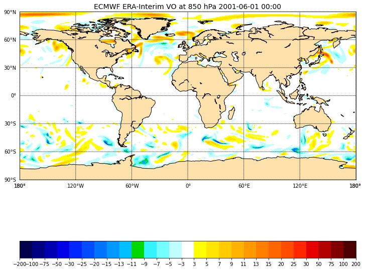
# 读取涡度变量
f = nc.Dataset('/home/mw/input/metos8969/metos/EI_VO_850hPa_Summer2001.nc', 'r')
lats = f.variables['lat'][:]
lons = f.variables['lon'][:]
VO = f.variables['VO'][0,0,:,:]*100000

fig = plt.figure(figsize=[12,15])  # 新窗口
ax = fig.add_subplot(1, 1, 1)  # 添加子图
ax.set_title('ECMWF ERA-Interim VO at 850 hPa 2001-06-01 00:00', fontsize=14)

map = Basemap(projection='merc',llcrnrlat=38,urcrnrlat=76,\
            llcrnrlon=-65,urcrnrlon=30, resolution='c', ax=ax)
map.drawcoastlines()
map.fillcontinents(color='#ffe2ab')
# 添加经纬度
map.drawparallels(np.arange(-90.,91.,20.))
map.drawmeridians(np.arange(-180.,181.,10.))
map.drawparallels(np.arange(-90.,120.,30.),labels=[1,0,0,0])
map.drawmeridians(np.arange(-180.,180.,60.),labels=[0,0,0,1])

# 经度范围设置为[-180,180]
VO,lons = shiftgrid(180.,VO,lons,start=False)
llons, llats = np.meshgrid(lons, lats)
x,y = map(llons,llats)
# 设置色阶
cmap = c.ListedColormap(['#00004c','#000080','#0000b3','#0000e6','#0026ff','#004cff',
                         '#0073ff','#0099ff','#00c0ff','#00d900','#33f3ff','#73ffff','#c0ffff',
                         (0,0,0,0),
                         '#ffff00','#ffe600','#ffcc00','#ffb300','#ff9900','#ff8000','#ff6600',
                         '#ff4c00','#ff2600','#e60000','#b30000','#800000','#4c0000'])
bounds=[-200,-100,-75,-50,-30,-25,-20,-15,-13,-11,-9,-7,-5,-3,3,5,7,9,11,13,15,20,25,30,50,75,100,200]
norm = c.BoundaryNorm(bounds, ncolors=cmap.N)
cs = map.contourf(x,y,VO, cmap=cmap, norm=norm, levels=bounds,shading='interp')

# 添加颜色条
fig.colorbar(cs, cmap=cmap, norm=norm, boundaries=bounds, ticks=bounds, ax=ax, orientation='horizontal')
f.close()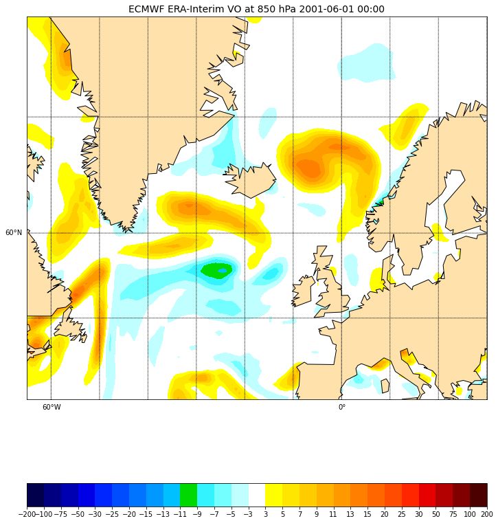
# 读取涡度变量
f = nc.Dataset('/home/mw/input/metos8969/metos/EI_VO_850hPa_Summer2001.nc', 'r')
lats = f.variables['lat'][:]
lons = f.variables['lon'][:]
VO = f.variables['VO'][0,0,:,:]*100000
fig = plt.figure(figsize=[12,15])  # 新窗口
ax = fig.add_subplot(1, 1, 1)  # 添加子图
ax.set_title('ECMWF ERA-Interim VO at 850 hPa 2001-06-01 00:00', fontsize=14)

map = Basemap(projection='merc', llcrnrlat=38, urcrnrlat=76, llcrnrlon=-65, urcrnrlon=30, resolution='c', ax=ax)
map.drawcoastlines()
map.fillcontinents(color='#ffe2ab')
# 添加经纬度
map.drawparallels(np.arange(-90.,91.,20.))
map.drawmeridians(np.arange(-180.,181.,10.))
map.drawparallels(np.arange(-90.,120.,30.),labels=[1,0,0,0])
map.drawmeridians(np.arange(-180.,180.,60.),labels=[0,0,0,1])

# 经度范围设置为[-180,180]
VO,lons = shiftgrid(180.,VO,lons,start=False)
llons, llats = np.meshgrid(lons, lats)
x,y = map(llons,llats)
# 设置色阶
cmap = c.ListedColormap(['#00004c','#000080','#0000b3','#0000e6','#0026ff','#004cff',
                         '#0073ff','#0099ff','#00c0ff','#00d900','#33f3ff','#73ffff','#c0ffff',
                         (0,0,0,0),
                         '#ffff00','#ffe600','#ffcc00','#ffb300','#ff9900','#ff8000','#ff6600',
                         '#ff4c00','#ff2600','#e60000','#b30000','#800000','#4c0000'])
bounds=[-200,-100,-75,-50,-30,-25,-20,-15,-13,-11,-9,-7,-5,-3,3,5,7,9,11,13,15,20,25,30,50,75,100,200]
norm = c.BoundaryNorm(bounds, ncolors=cmap.N)
cs = map.contourf(x,y,VO, cmap=cmap, norm=norm, levels=bounds,shading='interp')

# 添加颜色条
fig.colorbar(cs, cmap=cmap, norm=norm, boundaries=bounds, ticks=bounds, ax=ax, orientation='horizontal')
f.close()

# 读取海平面气压
f = nc.Dataset('/home/mw/input/metos8969/metos/EI_mslp_Summer2001.nc', 'r')
lats = f.variables['lat'][:]
lons = f.variables['lon'][:]
mslp = f.variables['MSL'][0,:,:]/100.0
# 经度范围设置为[-180,180]
mslp,lons = shiftgrid(180.,mslp,lons,start=False)
llons, llats = np.meshgrid(lons, lats)
x,y = map(llons,llats)
cs = map.contour(x,y,mslp, zorder=2, colors='black')
ax.clabel(cs, fmt='%.1f',fontsize=9, inline=1)
f.close()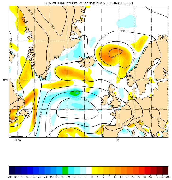
# 读取涡度变量
f = nc.Dataset('/home/mw/input/metos8969/metos/EI_VO_850hPa_Summer2001.nc', 'r')
lats = f.variables['lat'][:]
lons = f.variables['lon'][:]
VO = f.variables['VO'][0,0,:,:]*100000
fig = plt.figure(figsize=[12,15])  # 新窗口
ax = fig.add_subplot(1, 1, 1)  # 添加子图
ax.set_title('ECMWF ERA-Interim VO at 850 hPa 2001-06-01 00:00', fontsize=14)

map = Basemap(projection='merc',llcrnrlat=38,urcrnrlat=76, llcrnrlon=-65,urcrnrlon=30, resolution='c', ax=ax)
map.drawcoastlines()
map.fillcontinents(color='#ffe2ab')
# 添加经纬度
map.drawparallels(np.arange(-90.,91.,20.))
map.drawmeridians(np.arange(-180.,181.,10.))
map.drawparallels(np.arange(-90.,120.,30.),labels=[1,0,0,0])
map.drawmeridians(np.arange(-180.,180.,60.),labels=[0,0,0,1])

# 经度范围设置为[-180,180]
VO,lons = shiftgrid(180.,VO,lons,start=False)
llons, llats = np.meshgrid(lons, lats)
x,y = map(llons,llats)
# 设置色阶
cmap = c.ListedColormap(['#00004c','#000080','#0000b3','#0000e6','#0026ff','#004cff',
                         '#0073ff','#0099ff','#00c0ff','#00d900','#33f3ff','#73ffff','#c0ffff',
                         (0,0,0,0),
                         '#ffff00','#ffe600','#ffcc00','#ffb300','#ff9900','#ff8000','#ff6600',
                         '#ff4c00','#ff2600','#e60000','#b30000','#800000','#4c0000'])
bounds=[-200,-100,-75,-50,-30,-25,-20,-15,-13,-11,-9,-7,-5,-3,3,5,7,9,11,13,15,20,25,30,50,75,100,200]
norm = c.BoundaryNorm(bounds, ncolors=cmap.N) # cmap.N gives the number of colors of your palette
cs = map.contourf(x,y,VO, cmap=cmap, norm=norm, levels=bounds,shading='interp')

# 添加颜色条
fig.colorbar(cs, cmap=cmap, norm=norm, boundaries=bounds, ticks=bounds, ax=ax, orientation='horizontal')
f.close()

# 读取海平面气压
f = nc.Dataset('/home/mw/input/metos8969/metos/EI_mslp_Summer2001.nc', 'r')
lats = f.variables['lat'][:]
lons = f.variables['lon'][:]
mslp = f.variables['MSL'][0,:,:]/100.0
# 经度范围设置为[-180,180]
mslp,lons = shiftgrid(180.,mslp,lons,start=False)
llons, llats = np.meshgrid(lons, lats)
x,y = map(llons,llats)
cs = map.contour(x,y,mslp, zorder=2, colors='black')
ax.clabel(cs, fmt='%.1f',fontsize=9, inline=1)
f.close()

# 子图区域范围
llat=56
ulat=66
llon=-40
rlon=0

# 设置缩放比例及其子图位置
axins = zoomed_inset_axes(ax, 3, loc=1, bbox_to_anchor=(1.5, 1.0), bbox_transform=ax.figure.transFigure)

map.drawcoastlines(ax=axins)
map.fillcontinents(color='#ffe2ab', zorder=0, ax=axins)
# 添加经纬度
map.drawparallels(np.arange(-90.,120.,2.),labels=[0,0,0,0], ax=axins)
map.drawmeridians(np.arange(-180.,180.,10.),labels=[0,0,0,0], ax=axins)

# 设置子图显示范围
x1,y1 = map(llon, llat)
x2,y2 = map(rlon,ulat)
axins.set_xlim(x1, x2)
axins.set_ylim(y1, y2)
csins = map.contourf(x,y,VO, cmap=cmap, norm=norm, levels=bounds,shading='interp', zorder=1, ax=axins)
csins = map.contour(x,y,mslp,20,zorder=2, colors='black', ax=axins)
axins.clabel(csins, fontsize=14, inline=1,fmt = '%1.0f')
# 添加红色框线
axes = mark_inset(ax, axins, loc1=2, loc2=4, edgecolor='red', linestyle='dashed', linewidth=3)

# 读取台风轨迹数据
data = pd.read_csv('/home/mw/input/metos8969/metos/tracks_20010601.csv')
print(data)
xt, yt = map(np.array(data['lon']), np.array(data['lat']))
cols = ['blue' for i in range(xt.size)]
cols[0] = 'magenta'

# 添加黑色线
map.plot(xt,yt, '-', color='magenta', zorder=9, ax=axins, alpha=0.5, linewidth=4)
# 绘制颜色点
map.scatter(xt, yt, s=20**2, color=cols, edgecolor='#333333', zorder=10, ax=axins)
# 添加注释
for i, lpoint in enumerate(pandas.to_datetime(data["datetime"])):
   axins.annotate(' {0:d} h'.format(lpoint.hour), (xt[i],yt[i]),
               xytext=(15,0), textcoords='offset points',
               fontsize=24, color='darkblue')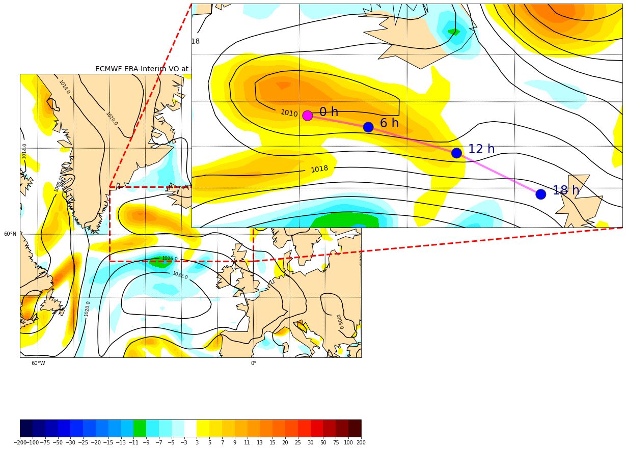
fig = plt.figure(figsize=(15,15))  # 新窗口
ax = fig.add_subplot(1, 1, 1)  # 添加子图
ax.set_title('Southern Norway and Sweden 29/02/2017  terra 1km', fontsize=14)

# 读取遥感影像数据
datafile = gdal.Open(r'/home/mw/input/metos8969/metos/Southern_Norway_and_Sweden.2017229.terra.1km.tif')
bnd1 = datafile.GetRasterBand(1).ReadAsArray()
bnd2 = datafile.GetRasterBand(2).ReadAsArray()
bnd3 = datafile.GetRasterBand(3).ReadAsArray()
nx = datafile.RasterXSize
ny = datafile.RasterYSize

img = np.dstack((bnd1, bnd2, bnd3))
gt = datafile.GetGeoTransform()
proj = datafile.GetProjection()

print("Geotransform",gt)
print("proj=", proj)
xres = gt[1]
yres = gt[5]

# 获取地图范围
xmin = gt[0] + xres * 0.5
xmax = gt[0] + (xres * nx) - xres * 0.5
ymin = gt[3] + (yres * ny) + yres * 0.5
ymax = gt[3] - yres * 0.5
print("xmin=", xmin,"xmax=", xmax,"ymin=",ymin, "ymax=", ymax)

map = Basemap(projection='cyl',llcrnrlat=ymin,urcrnrlat=ymax, llcrnrlon=xmin,urcrnrlon=xmax , resolution='i', ax=ax)
map.imshow(img, origin='upper', ax=ax)
map.drawcountries(color='blue', linewidth=1.5, ax=ax)
map.drawcoastlines(linewidth=1.5, color='red', ax=ax)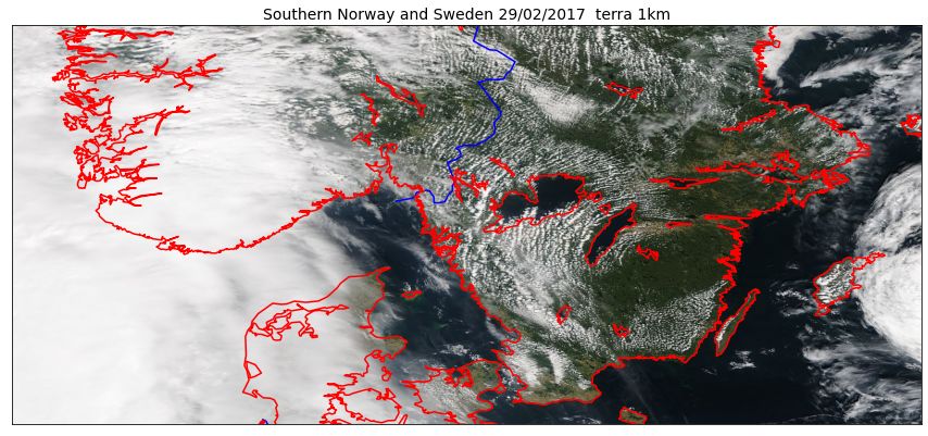
fig = plt.figure(figsize=(15,15))  # 新窗口
ax = fig.add_subplot(1, 1, 1)  # 添加子图
ax.set_title('Southern Norway and Sweden 29/02/2017  terra 1km', fontsize=14)

# 读取遥感影像数据
datafile = gdal.Open(r'/home/mw/input/metos8969/metos/Southern_Norway_and_Sweden.2017229.terra.1km.tif')
bnd1 = datafile.GetRasterBand(1).ReadAsArray()
nx = datafile.RasterXSize
ny = datafile.RasterYSize

gt = datafile.GetGeoTransform()
proj = datafile.GetProjection()

print("Geotransform",gt)
print("proj=", proj)
xres = gt[1]
yres = gt[5]

# 获取地图范围
xmin = gt[0] + xres * 0.5
xmax = gt[0] + (xres * nx) - xres * 0.5
ymin = gt[3] + (yres * ny) + yres * 0.5
ymax = gt[3] - yres * 0.5
print("xmin=", xmin,"xmax=", xmax,"ymin=",ymin, "ymax=", ymax)
(lon_source,lat_source) = np.mgrid[xmin:xmax+xres:xres, ymax+yres:ymin:yres]
print(xmin,xmax+xres,xres, ymax+yres,ymin,yres)
# 设置cyl投影
map = Basemap(projection='cyl',llcrnrlat=ymin,urcrnrlat=ymax,llcrnrlon=xmin,urcrnrlon=xmax , resolution='i', ax=ax)
map.pcolormesh(lon_source,lat_source,bnd1.T, cmap='bone')
map.drawcountries(color='blue', linewidth=1.5, ax=ax)
map.drawcoastlines(linewidth=1.5, color='red', ax=ax)
fig = plt.figure(figsize=(15,15))  # 新窗口
ax = fig.add_subplot(1, 1, 1)  # 添加子图
ax.set_title('Southern Norway and Sweden 29/02/2017  terra 1km', fontsize=14)

# 读取遥感影像数据
datafile = gdal.Open(r'/home/mw/input/metos8969/metos/Southern_Norway_and_Sweden.2017229.terra.1km.tif')
bnd1 = datafile.GetRasterBand(1).ReadAsArray()
bnd2 = datafile.GetRasterBand(2).ReadAsArray()
bnd3 = datafile.GetRasterBand(3).ReadAsArray()
nx = datafile.RasterXSize
ny = datafile.RasterYSize

rgb = np.dstack((bnd1/bnd1.max(), bnd2/bnd2.max(), bnd3/bnd3.max()))
color_tuple = rgb.transpose((1,0,2)).reshape((rgb.shape[0]*rgb.shape[1],rgb.shape[2]))
gt = datafile.GetGeoTransform()
proj = datafile.GetProjection()

print("Geotransform",gt)
print("proj=", proj)
xres = gt[1]
yres = gt[5]

# 获取地图范围
xmin = gt[0] + xres * 0.5
xmax = gt[0] + (xres * nx) - xres * 0.5
ymin = gt[3] + (yres * ny) + yres * 0.5
ymax = gt[3] - yres * 0.5
print("xmin=", xmin,"xmax=", xmax,"ymin=",ymin, "ymax=", ymax)
(lon_source,lat_source) = np.mgrid[xmin:xmax+xres:xres, ymax+yres:ymin:yres]
print(xmin,xmax+xres,xres, ymax+yres,ymin,yres)
# 设置merc投影
map = Basemap(projection='merc',llcrnrlat=ymin,urcrnrlat=ymax,llcrnrlon=xmin,urcrnrlon=xmax , resolution='i', ax=ax)
x,y = map(lon_source, lat_source)
print("shape lon and lat_source: ", lon_source.shape, lat_source.shape,bnd1.T.shape)
map.pcolormesh(x,y,bnd1.T,color=color_tuple)
map.drawcountries(color='blue', linewidth=1.5, ax=ax)
map.drawcoastlines(linewidth=1.5, color='red', ax=ax)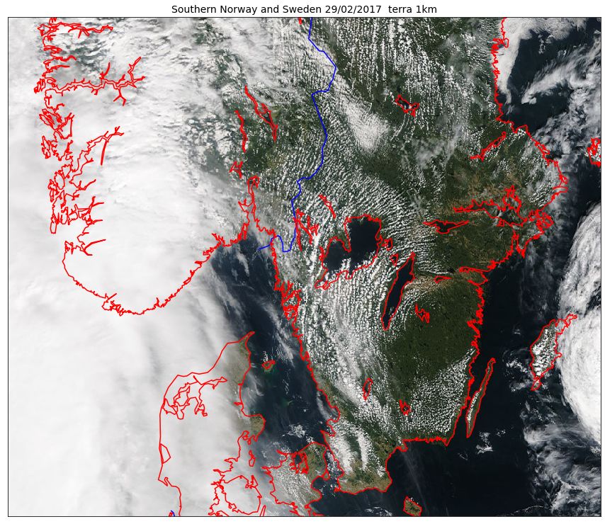
fig = plt.figure(figsize=[12,15])  # 新窗口
ax = fig.add_subplot(1, 1, 1)      # 添加子图
map = Basemap(llcrnrlon=-1.0,urcrnrlon=40.,llcrnrlat=55.,urcrnrlat=75., resolution='i', projection='lcc', lat_1=65., lon_0=5.)
map.drawmapboundary(fill_color='aqua')
map.fillcontinents(color='#ffe2ab',lake_color='aqua')
map.drawcoastlines()
norway_roads= map.readshapefile('/home/mw/input/metos8969/metos/Norway_railways/railways', 'railways')
plt.show()
fig = plt.figure(figsize=[12,15])  # 新窗口
ax = fig.add_subplot(1, 1, 1)      # 添加子图
map = Basemap(llcrnrlon=-1.0,urcrnrlon=40.,llcrnrlat=55.,urcrnrlat=75.,resolution='i', projection='lcc', lat_1=65., lon_0=5.)
map.fillcontinents(color='#ffe2ab')
map.drawcoastlines()
norway_roads= map.readshapefile('/home/mw/input/metos8969/metos/Norway_railways/railways', 'railways', color='red',linewidth=1.5)
plt.show()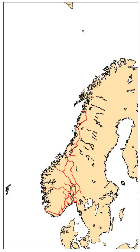
fig = plt.figure(figsize=[12,15])  # 新窗口
ax = fig.add_subplot(1, 1, 1)      # 添加子图
map = Basemap(llcrnrlon=-1.0,urcrnrlon=40.,llcrnrlat=55.,urcrnrlat=75., resolution='i', projection='lcc', lat_1=65., lon_0=5.)
map.drawmapboundary(fill_color='white')
map.fillcontinents(color='#ffe2ab', zorder=0, ax=ax)
map.drawcoastlines()
norway_natural= map.readshapefile('/home/mw/input/metos8969/metos/NOR_adm/NOR_adm', 'NOR_adm', color='blue',  drawbounds=True)
plt.show()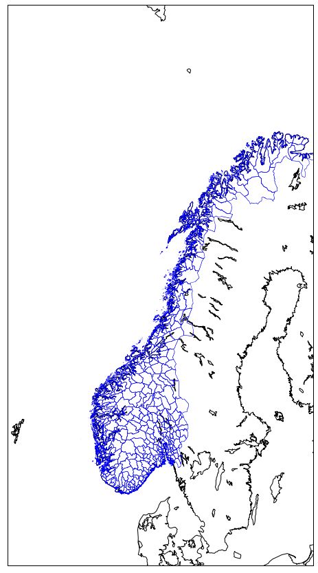
shapedata = ogr.Open('/home/mw/input/metos8969/metos/NOR_adm')
nblayer = shapedata.GetLayerCount()
print("Number of layers: ", nblayer)
layer = shapedata.GetLayer()
nor_adm = []
for i in range(layer.GetFeatureCount()):
    feature = layer.GetFeature(i)
    name_1 = feature.GetField("NAME_1")
    id_1 = feature.GetField("ID_1")
    geometry = feature.GetGeometryRef()
    nor_adm.append([i,name_1,id_1, geometry.GetGeometryName(), geometry.Centroid().ExportToWkt()])
for i in range(0,len(nor_adm),20):
    print(nor_adm[i])

fig = plt.figure(figsize=[12,15])
ax = fig.add_subplot(111)
map = Basemap(llcrnrlon=-1.0,urcrnrlon=40.,llcrnrlat=55.,urcrnrlat=75., resolution='i', projection='lcc', lat_1=65., lon_0=5.)
map.drawmapboundary(fill_color='white')
map.fillcontinents(color='#ffe2ab', zorder=0, ax=ax)
map.drawcoastlines()
map.readshapefile('/home/mw/input/metos8969/metos/NOR_adm/NOR_adm', 'NOR_adm', drawbounds = False)
patches = []
color_values = np.zeros(len(map.NOR_adm))
for i, info, shape in zip(range(len(map.NOR_adm_info)),map.NOR_adm_info, map.NOR_adm):
        patches.append( Polygon(np.array(shape), True))
        color_values[i] = info['ID_1']
col = PatchCollection(patches, linewidths=1., zorder=2)
col.set(array=color_values, cmap='jet')
ax.add_collection(col)
三、时空数据的基本分析
导入模块
import netCDF4
import numpy as np
from scipy.cluster.vq import *
from matplotlib import colors as c
import matplotlib.pyplot as plt
from scipy.spatial import distance
from skimage import measure
import geopandas as gpd
from fiona.crs import from_epsg
from shapely import geometry
from mpl_toolkits.basemap import Basemap
K-Means聚类
K均值是聚类分析中广泛使用的方法。但是,仅当许多假设对数据集有效时,此方法才有效:
-
k-means 假设每个属性(变量)的分布方差是球形的;
-
所有变量具有相同的方差;
-
所有 k 个聚类的先验概率相同,即每个聚类的观测值数大致相等;
如果违反了这3个假设中的任何一个,那么k均值将不正确。
使用K均值时必须做出的重大决定是先验地选择聚类的数量。但是,正如我们将在下面看到的,此选择至关重要,并且对结果有很大的影响:
f = netCDF4.Dataset('/home/mw/input/metos8969/metos/tpw_v07r01_200910.nc4.nc', 'r')
lats = f.variables['latitude'][:]
lons = f.variables['longitude'][:]
pw = f.variables['precipitable_water'][0,:,:]

f.close()
# Flatten image to get line of values
flatraster = pw.flatten()
flatraster.mask = False
flatraster = flatraster.data

# Create figure to receive results
fig = plt.figure(figsize=[20,7])
fig.suptitle('K-Means Clustering')

# In first subplot add original image
ax = plt.subplot(241)
ax.axis('off')
ax.set_title('Original Image\nMonthly Average Precipitable Water\n over Ice-Free Oceans (kg m-2)')
original=ax.imshow(pw, cmap='rainbow', interpolation='nearest', aspect='auto', origin='lower')
plt.colorbar(original, cmap='rainbow', ax=ax, orientation='vertical')
# In remaining subplots add k-means clustered images
# Define colormap
list_colors=['blue','orange', 'green', 'magenta', 'cyan', 'gray', 'red', 'yellow']
for i in range(7):
    print("Calculate k-means with ", i+2, " clusters.")

    #This scipy code clusters k-mean, code has same length as flattened
    # raster and defines which cluster the value corresponds to
    centroids, variance = kmeans(flatraster.astype(float), i+2)
    code, distance = vq(flatraster, centroids)

    #Since code contains the clustered values, reshape into SAR dimensions
    codeim = code.reshape(pw.shape[0], pw.shape[1])

    #Plot the subplot with (i+2)th k-means
    ax = plt.subplot(2,4,i+2)
    ax.axis('off')
    xlabel = str(i+2) , ' clusters'
    ax.set_title(xlabel)
    bounds=range(0,i+2)
    cmap = c.ListedColormap(list_colors[0:i+2])
    kmp=ax.imshow(codeim, interpolation='nearest', aspect='auto', cmap=cmap,  origin='lower')
    plt.colorbar(kmp, cmap=cmap,  ticks=bounds, ax=ax, orientation='vertical')
plt.show()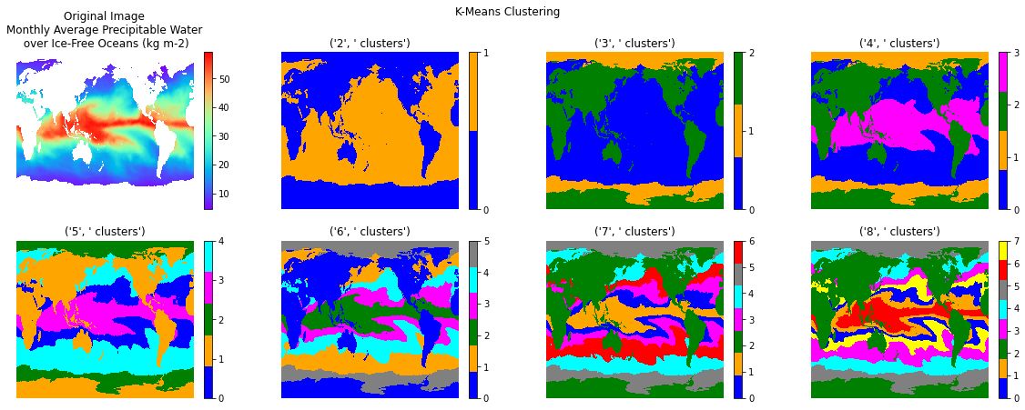
np.random.seed((1000,2000))

f = netCDF4.Dataset('/home/mw/input/metos8969/metos/tpw_v07r01_200910.nc4.nc', 'r')
lats = f.variables['latitude'][:]
lons = f.variables['longitude'][:]
pw = f.variables['precipitable_water'][0,:,:]

f.close()
# Flatten image to get line of values
flatraster = pw.flatten()
flatraster.mask = False
flatraster = flatraster.data


# In first subplot add original image
fig, (ax1, ax2, ax3)  = plt.subplots(3, sharex=True)

# Create figure to receive results
fig.set_figheight(20)
fig.set_figwidth(15)

fig.suptitle('K-Means Clustering')
ax1.axis('off')
ax1.set_title('Original Image\nMonthly Average Precipitable Water\n over Ice-Free Oceans (kg m-2)')
original=ax1.imshow(pw, cmap='rainbow', interpolation='nearest', aspect='auto', origin='lower')
plt.colorbar(original, cmap='rainbow', ax=ax1, orientation='vertical')
# In remaining subplots add k-means clustered images
# Define colormap
list_colors=['blue','orange', 'green', 'magenta', 'cyan', 'gray', 'red', 'yellow']

print("Calculate k-means with 6 clusters.")

#This scipy code classifies k-mean, code has same length as flattened
# raster and defines which cluster the value corresponds to
centroids, variance = kmeans(flatraster.astype(float), 6)
code, distance = vq(flatraster, centroids)

#Since code contains the clustered values, reshape into SAR dimensions
codeim = code.reshape(pw.shape[0], pw.shape[1])

#Plot the subplot with 4th k-means
ax2.axis('off')
xlabel = '6 clusters'
ax2.set_title(xlabel)
bounds=range(0,6)
cmap = c.ListedColormap(list_colors[0:6])
kmp=ax2.imshow(codeim, interpolation='nearest', aspect='auto', cmap=cmap,  origin='lower')
plt.colorbar(kmp, cmap=cmap,  ticks=bounds, ax=ax2, orientation='vertical')

#####################################
thresholded = np.zeros(codeim.shape)
thresholded[codeim==3]=1
thresholded[codeim==4]=2

#Plot only values == 5
ax3.axis('off')
xlabel = 'Keep the fifth cluster only'
ax3.set_title(xlabel)
bounds=range(0,2)
cmap = c.ListedColormap(['white', 'green', 'cyan'])
kmp=ax3.imshow(thresholded, interpolation='nearest', aspect='auto', cmap=cmap,  origin='lower')
plt.colorbar(kmp, cmap=cmap,  ticks=bounds, ax=ax3, orientation='vertical')

plt.show()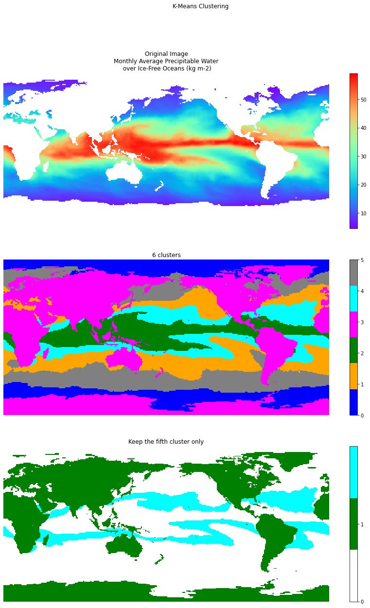
保存等值线轮廓
为了保存生成的等值线,我们需要获取等值线的每个点的坐标并创建一个面。在lat/lon中添加坐标的计算,并使用Geopandas包将它们存储在shapefile中。
from scipy.spatial import distance
# 寻找等值线
contours = measure.find_contours(thresholded, 1.0)
# 图像展示
fig = plt.figure(figsize=[20,7])
ax = plt.subplot()
ax.set_title('Original Image\nMonthly Average Precipitable Water\n over Ice-Free Oceans (kg m-2)')
original=ax.imshow(pw, cmap='rainbow', interpolation='nearest', aspect='auto', origin='lower')
plt.colorbar(original, cmap='rainbow', ax=ax, orientation='vertical')
for n, contour in enumerate(contours):
    dists = distance.cdist(contour, contour, 'euclidean')
    if dists.max() > 200:
        ax.plot(contour[:, 1], contour[:, 0], linewidth=2, color='black')
        print(dists.max())
# 寻找等值线
contours = measure.find_contours(thresholded, 1.0)
# 创建空的的GeoDataFrame
newdata = gpd.GeoDataFrame()
# 创建一个字段
newdata['geometry'] = None
# 设置地理坐标
newdata.crs = from_epsg(4326)
# 图像展示
fig = plt.figure(figsize=[20,7])
ax = plt.subplot()
ax.set_title('Original Image\nMonthly Average Precipitable Water\n over Ice-Free Oceans (kg m-2)')
original = ax.imshow(pw, cmap='rainbow', interpolation='nearest', aspect='auto', origin='lower')
plt.colorbar(original, cmap='rainbow', ax=ax, orientation='vertical')
ncontour = 0
for n, contour in enumerate(contours):
    dists = distance.cdist(contour, contour, 'euclidean')
    if dists.max() > 200:
        ax.plot(contour[:, 1], contour[:, 0], linewidth=2, color='black')
        coords = []
        for c in contour:
            if int(c[0]) == c[0]:
                lat = lats[int(c[ 0])]
            else:
                lat = (lats[int(c[ 0])] + lats[int(c[0])+1])/2.0
            if int(c[1]) == c[1]:
                lon = lons[int(c[ 1])]
            else:
                lon = (lons[int(c[ 1])] + lons[int(c[1])+1])/2.0
            coords.append([lon,lat])

        poly = geometry.Polygon([[c[0], c[1]] for c in coords])
        newdata.loc[ncontour, 'geometry'] = poly
        newdata.loc[ncontour,'idx_name'] = 'contour_' + str(ncontour)
        print(ncontour)
        print(dists.max())
        ncontour += 1
# 写入数据
newdata.to_file('contour_test.shp')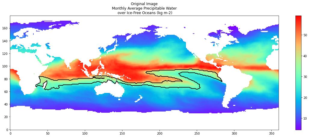
fig = plt.figure(figsize=[12,15])  # 新窗口
ax = fig.add_subplot(1, 1, 1)  # 添加子图
map = Basemap(projection='cyl',llcrnrlat=-90,urcrnrlat=90,llcrnrlon=0,urcrnrlon=360,resolution='c')
map.drawmapboundary(fill_color='aqua')
map.fillcontinents(color='#ffe2ab',lake_color='aqua')
map.drawcoastlines()
contour_test= map.readshapefile('contour_test', 'contour_test', linewidth=2.0, color="red")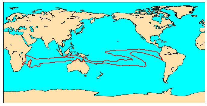
四、大型数据集的处理
我们在处理小容量数据文件时是相对快速且便捷的,但是对于大容量数据文件,在笔记本上运行很可能出现内存溢出问题。因此,我们需要转移到大型服务器或云计算平台,并且可以通过并行计算等方法加快数据处理工作,并节约内存开销。
导入模块
import netCDF4 as nc
import numpy as np
import h5py
import os
import dask.array as da
from IPython.display import Image
import dask.array as da
读取数据
# 对数据进行切片处理(循环方式)
d = nc.Dataset('/home/mw/input/metos8969/metos/EI_VO_850hPa_Summer2001.nc', 'a')
data = d.variables['VO']
t = d.variables['time']
last_time = t[t.size-1]
VO = data[0,:,:,:]
appendvar = d.variables['VO']
for nt in range(t.size,t.size+50):
    VO += 0.1 * np.random.randn()
    last_time += 6.0
    appendvar[nt] = VO
    t[nt] = last_time
d.close()


# 对数据进行切片处理(索引方式)
d = nc.Dataset('/home/mw/input/metos8969/metos/EI_VO_850hPa_Summer2001.nc', 'r')
data = d.variables['VO']
slice_t = data[:,0,30,30]


d = nc.Dataset('/home/mw/input/metos8969/metos/EI_VO_850hPa_Summer2001.nc', 'r')
print(d)
d.close()
压缩文件
在写入数据集时使用 netCDF-4 / HDF-5 数据压缩以节省磁盘空间。NetCDF4 和 HDF5 提供了简单的方法来压缩数据。创建变量时,可以通过设置关键字参数 zlib=True 来打开数据压缩,但也可以选择数据的压缩率和精度:
-
关键字参数切换压缩比和速度。complevel选项范围从 1 到 9(1 表示压缩最少时最快的选项,9 表示压缩次数最多的最慢选项,默认值为 4)
-
可以使用least_significant_digit关键字参数指定数据的精度。浮点数的存储精度通常比浮点数所表示的数据高得多,尤其是在处理观测值时。尾随数字会占用大量空间,可能不相关。通过指定最低有效位,可以进一步增强数据压缩。这只会给netCDF更多的自由,当它把数据打包到你的硬盘上。例如,知道温度仅精确到大约0.005°C,因此保留前4位数字是有意义的
# 源文件
src_file = '/home/mw/input/metos8969/metos/EI_VO_850hPa_Summer2001.nc'
# 目标文件
trg_file = 'compressed.nc'
# 读取源文件
src = nc.Dataset(src_file)
# 创建目标文件
trg = nc.Dataset(trg_file, mode='w')
# 创建维度
for name, dim in src.dimensions.items():
trg.createDimension(name, len(dim) if not dim.isunlimited() else None)
# 拷贝属性
trg.setncatts({a:src.getncattr(a) for a in src.ncattrs()})
# 创建变量
for name, var in src.variables.items():
trg.createVariable(name, var.dtype, var.dimensions, zlib=True)
# 拷贝变量属性
trg.variables[name].setncatts({a:var.getncattr(a) for a in var.ncattrs()})
# 拷贝变量值
trg.variables[name][:] = src.variables[name][:]
# 保存文件
trg.close()
src.close()
# 读取he5文件
f = h5py.File('/home/mw/input/metos8969/metos/OMI-Aura_L3-OMTO3e_2017m0105_v003-2017m0203t091906.he5', 'r')
dset = f['/HDFEOS/GRIDS/OMI Column Amount O3/Data Fields/ColumnAmountO3']
print(dset.shape)
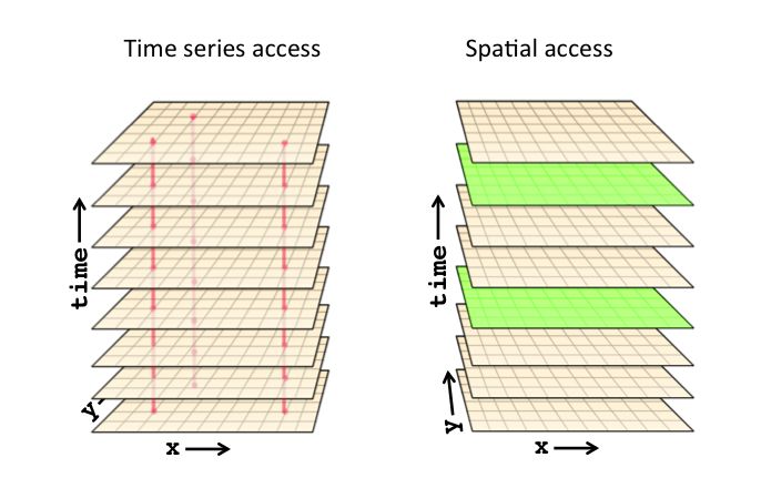
print(type(dset))并行计算:Dask
大型数据集的处理通常会遇到以下问题:
-
文件太大,无法放入内存
-
数据处理时间太长,无法在单个处理器上运行
-
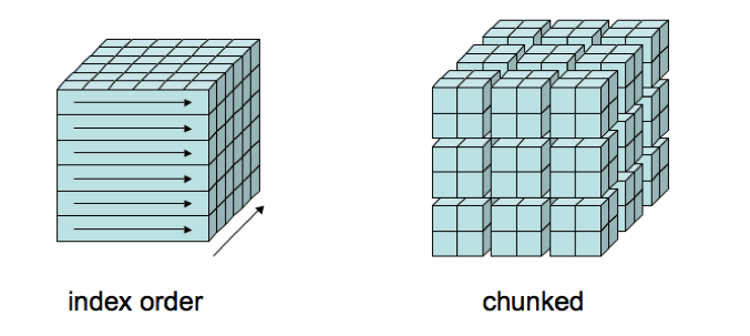
数据分块非常强大,但是编写程序,我们既对数据进行分块又进行处理可能会很麻烦。
为了加快我们的处理速度,我们需要使用多个处理器,因此我们需要一个足够简单和高效的框架。Dask是一个python库,有助于并行化大块数据的计算。
d_chunks = da.from_array(dset, chunks=(720, 144))
mx = d_chunks.max()
# 可视化并行任务流程
# 从下往上看图片,数据被划分为10个区块,最终得到整个字段的最大值
mx.visualize()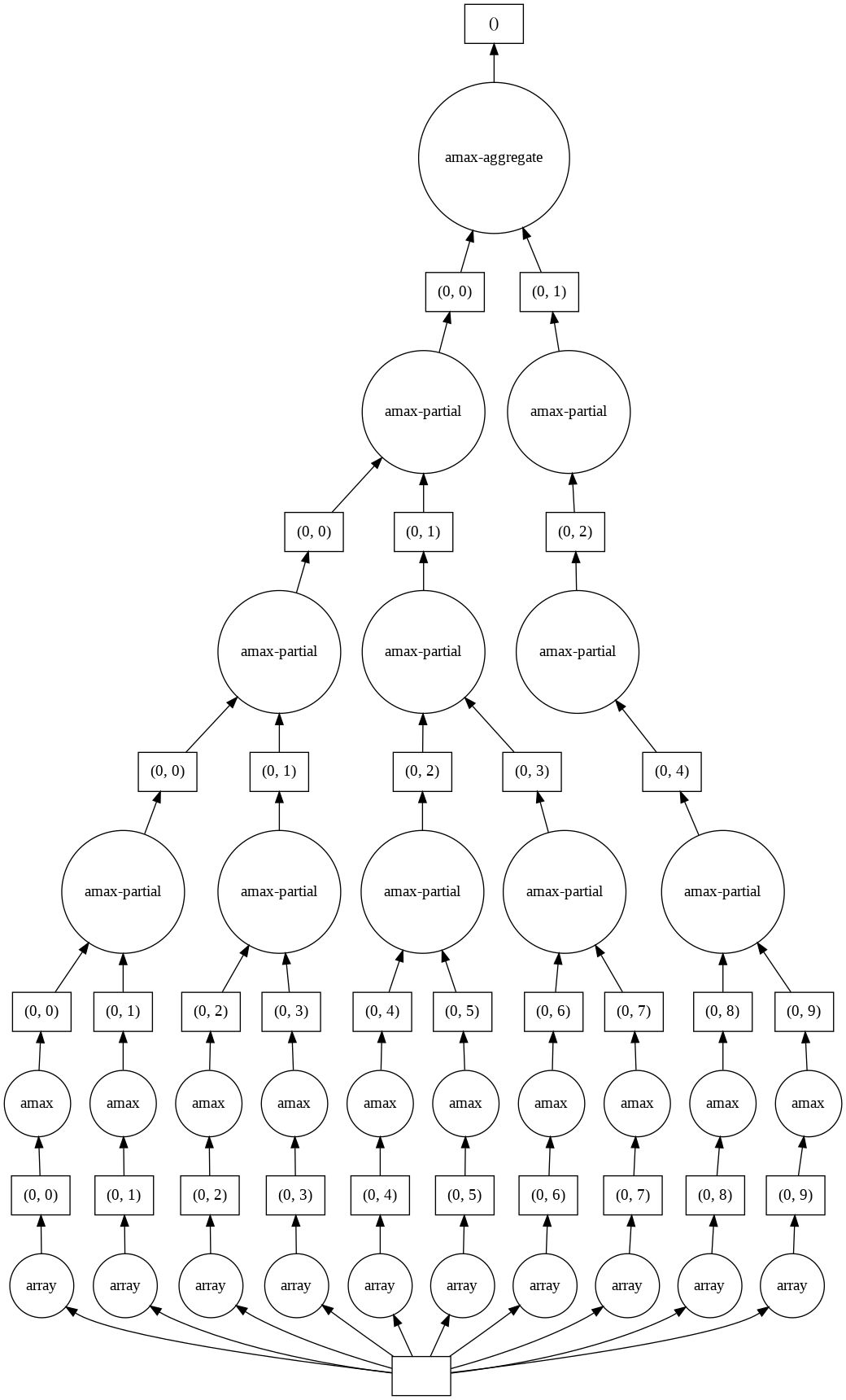
# 并行计算
mx.compute()


f = Dataset('/home/mw/input/metos8969/metos/EI_VO_850hPa_Summer2001.nc')
VO = da.from_array(f.variables['VO'], chunks=(63,1,256,512))
print(VO.shape)
VOmean = VO.mean()
print(VOmean)
#VOmean.compute()
# 可视化并行任务流程(计算平均值)
VOmean.visualize()
#(VO - VO.mean()).compute()
# 可视化并行任务流程(计算标准差)
(VO - VO.mean()).visualize()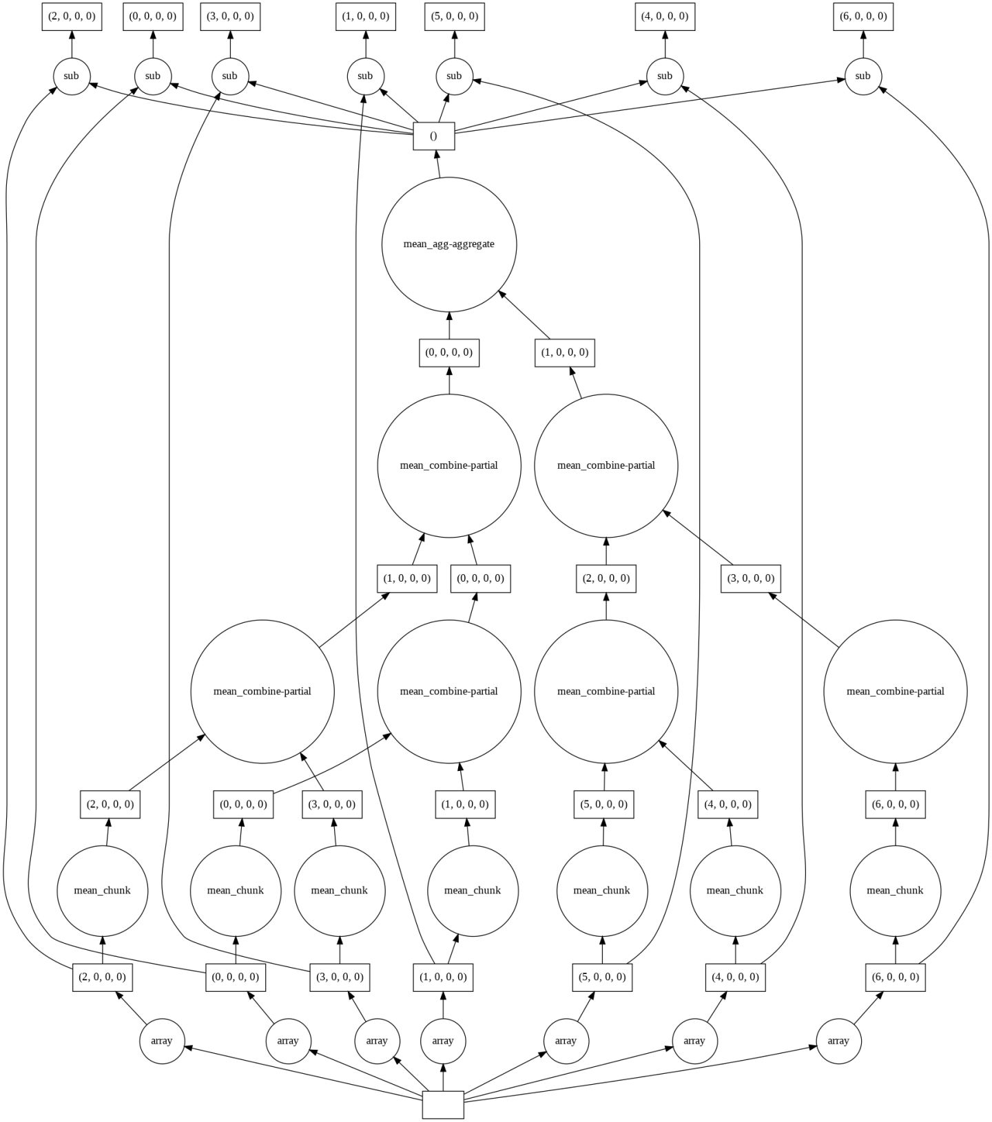
数据上传至和鲸社区数据集 | Python气象时空数据处理(演示数据)
获得代码运行环境,一键运行项目请点击>>快速入门基于Python的时空数据分析快速入门基于Python的时空数据分析