【数据挖掘】使用LightGBM和RandomForest对房屋出租价格的预测

1.摘要

房屋出租价格预测是一个很现实，也很接地气的问题。本文通过爬虫获取的上海出租房屋价格数据，包括50个房屋特征，通过建模分析得到，房屋特征与出租价格之间的相关性。熟悉了本篇数据挖掘的过程，也可以用到其他房产公司的房屋价格统计，买房时的价格预测和定位，或者做房屋数据分析时的统计等方面。通过该案例，不会讲解看房买房租房的方方面面，但可以给读者一个启发，通过这些代码和数据挖掘方法，达到解决问题的目的。
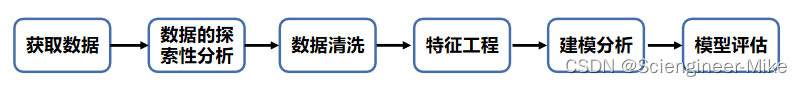
本篇展示了数据分析与挖掘的整个流程，并使用lightGBM和随机森林算法分别测试集房屋数据进行预测对比，预测效果基本吻合。让大家了解如何到对房屋数据中的字符型数据和数值型数据进行分析，如何使用SelectKBest筛选特征，如何建立机器学习算法模型。本篇的分析流程包括：

数据的探索性分析虽然在整个数据挖掘过程看不到具体体现，但它对我们后面的数据清洗、特征工程起着十分重要的作用。
数据探索性分析比较耗时，我们在这里只展示分析结果。
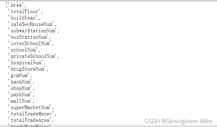
数据如下：

有需要的同学可以私聊我，获取分析数据。

2.数据分析与挖掘的整个过程

首先，导入相应的包，并导入数据。

# 导入相应的包
import pandas as pd
import numpy as np
import lightgbm as lgb
import matplotlib.pyplot as plt
from sklearn.feature_selection import SelectKBest,f_regression
from sklearn.ensemble import RandomForestRegressor
from sklearn.model_selection import train_test_split
from sklearn.metrics import r2_score

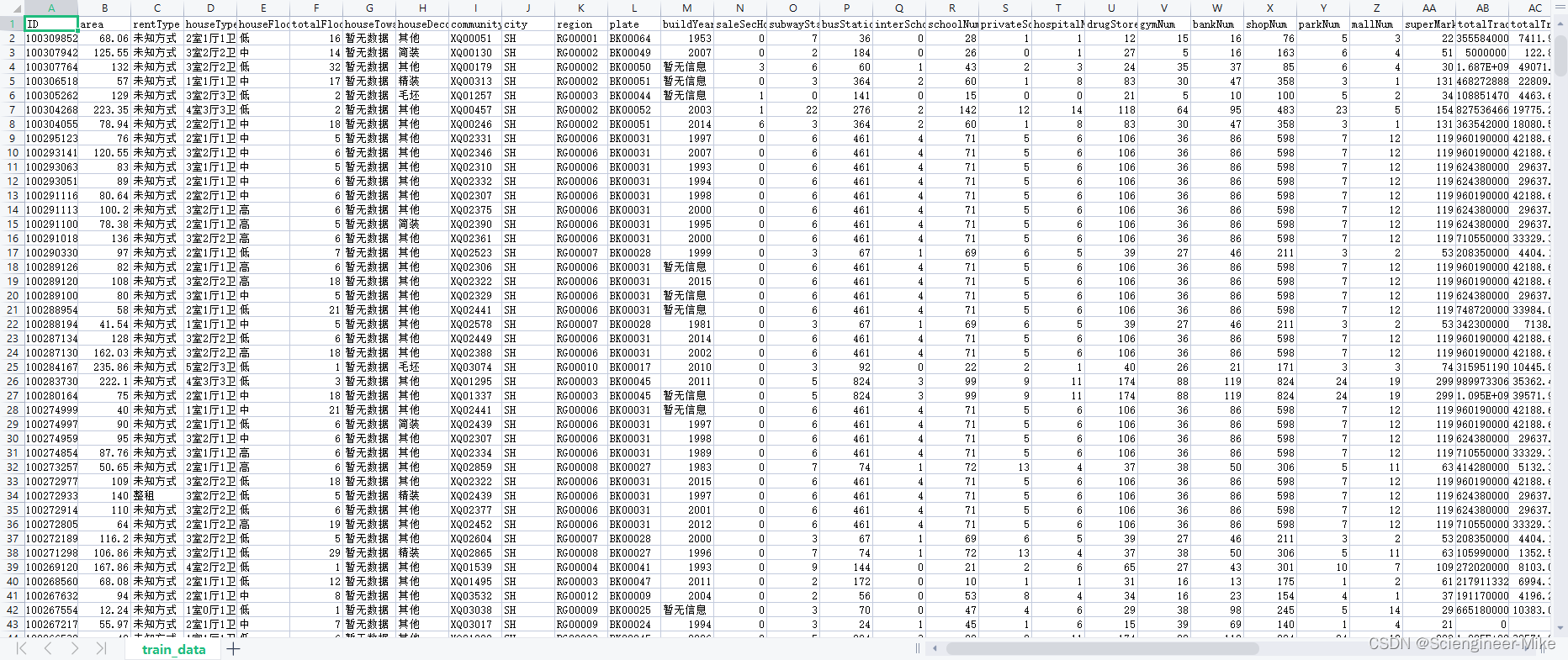
train = pd.read_csv("./train_data.csv")
test = pd.read_csv("./test_a.csv")

查看train和test数据，可以发现，train具有51列，test具有50列，train多了一个“tradeMoney”的标签值。
接下俩，进行数据清洗。
首先，房屋面积大于700和交易交割大于30000为异常值，删除处理，部分缺失值用众数进行填充。

#1.房屋面积要小于700,房屋交易价格低于30000，否则数据为异常数据
train = train[(train["area"]<=700) & (train["tradeMoney"]<=30000)]
# 2.特征rentType为”-“，转换为未知方式，方便后续处理
train[train["rentType"]=="--"]["rentType"] = '未知方式'
test[test["rentType"]=="--"]["rentType"] = '未知方式'
# 3.特征“buildYear”为“暂无信息”，用众数1994填充
train["buildYear"] = np.where(train["buildYear"]=="暂无信息",1994,train["buildYear"])
train["buildYear"] = train["buildYear"].astype("int")
test["buildYear"] = np.where(test["buildYear"]=="暂无信息",1994,test["buildYear"])
test["buildYear"] = test["buildYear"].astype("int")

然后，我们提取其中的分类特征，将其转化为category类型。

columns = ["rentType","houseFloor","houseToward","houseDecoration","communityName","region","plate"]
for col in columns:
    train[col] = train[col].astype("category")
    test[col] = test[col].astype("category")

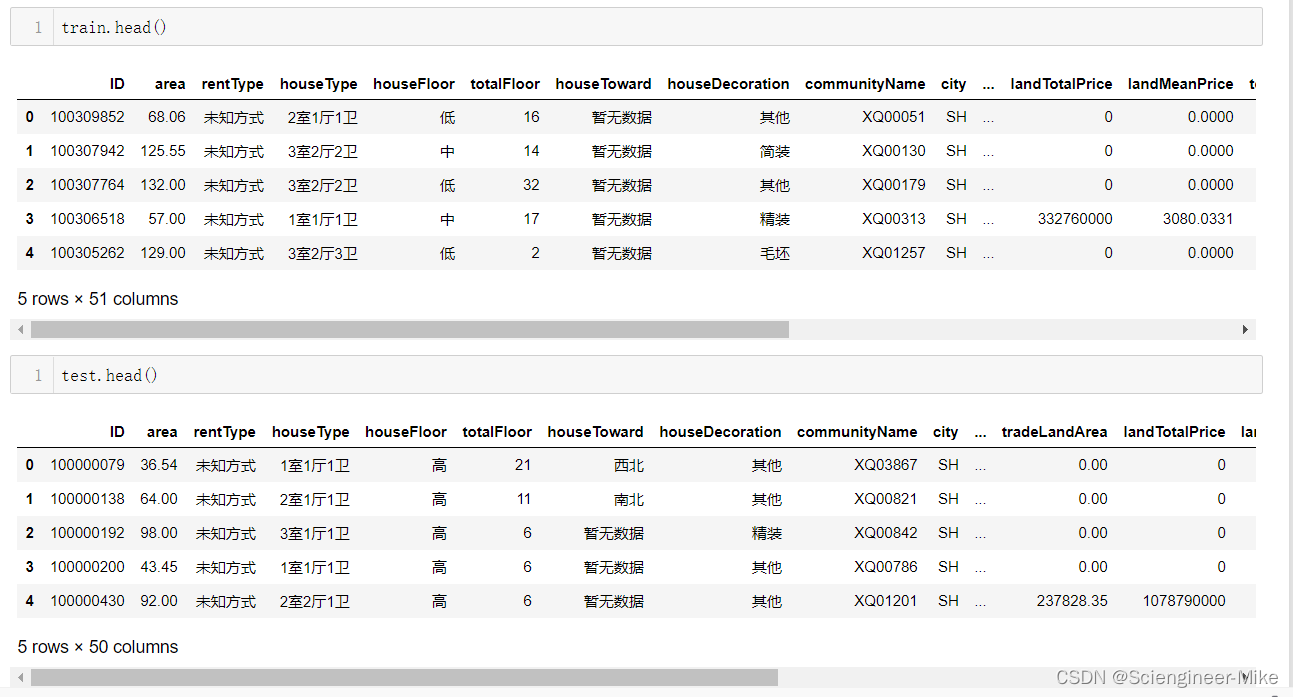
查看缺失值

df = train.isnull().sum().to_frame()
df[df[0]>0]

这两个特征为数值型特征，用均值进行填充。

# 缺失值使用均值来填充
train["pv"].fillna(train["pv"].mean(),inplace=True)
train["uv"].fillna(train["uv"].mean(),inplace=True)
test["pv"].fillna(test["pv"].mean(),inplace=True)
test["uv"].fillna(test["uv"].mean(),inplace=True)

删除无用的特征“ID",“city”

train.drop(["ID","city"],axis=1,inplace=True)
test.drop(["ID","city"],axis=1,inplace=True)

对houseType为”XX室XX厅XX卫“，这样的特征进行分解，创造特征。
—train处理

# 对train进行处理
# 将houseType转化为房间数room,厅数parlor,卫生间数bathroom
train["_roomNum"] = train["houseType"].apply(lambda x:int(x.split('室')[0]))
train["_bathroomNum"] = train["houseType"].apply(lambda x:int(x.split('厅')[1][0]))
train["_parlorNum"] = train["houseType"].apply(lambda x:int(x.split('室')[1][0]))
del train["houseType"]
# 合并房间总数
train["_roomNumSum"] = train["_roomNum"] + train["_bathroomNum"] + train["_parlorNum"]
# 合并数据
train["_trafficStationNums"] = train["subwayStationNum"] + train["busStationNum"]
train["_schoolNums"] = train["interSchoolNum"] + train["schoolNum"] + train["privateSchoolNum"]
train["_lifeHouseNums"] = train["gymNum"] + train["parkNum"] + train["bankNum"] + train["shopNum"] + train["mallNum"] + train["superMarketNum"]
# 将时间设置为交易月份
train["_tradeMonth"] = train["tradeTime"].apply(lambda x:int(x.split("/")[1]))

—test处理

# 对test进行处理
# 将houseType转化为房间数room,厅数parlor,卫生间数bathroom
test["_roomNum"] = test["houseType"].apply(lambda x:int(x.split('室')[0]))
test["_bathroomNum"] = test["houseType"].apply(lambda x:int(x.split('厅')[1][0]))
test["_parlorNum"] = test["houseType"].apply(lambda x:int(x.split('室')[1][0]))
del test["houseType"]
# 合并房间总数
test["_roomNumSum"] = test["_roomNum"] + test["_bathroomNum"] + test["_parlorNum"]
# 合并数据
test["_trafficStationNums"] = test["subwayStationNum"] + test["busStationNum"]
test["_schoolNums"] = test["interSchoolNum"] + test["schoolNum"] + test["privateSchoolNum"]
test["_lifeHouseNums"] = test["gymNum"] + test["parkNum"] + test["bankNum"] + test["shopNum"] + test["mallNum"] + test["superMarketNum"]
test["_tradeMonth"] = test["tradeTime"].apply(lambda x:int(x.split("/")[1]))

分离出标签值和特征值。

target = train.pop("tradeMoney")
features = train.columns

其中数据型特征和分类型特征如下：

# 分类特征
categorical_columns = ["rentType","houseFloor","houseToward","houseDecoration","region","plate"]
# 数值特征
num_features = []
for i in features:
    if train[i].dtype in ["int32","int64","float64"]:
        num_features.append(i)
num_features

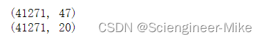
通过SelectKBest选取最重要的20个特征。

X,y = train[num_features],target
print(X.shape)
X_new = SelectKBest(f_regression,k=20).fit_transform(X,y)
print(X_new.shape)

得到这20个特征的索引，方便后续处理。

# 得到所需要的索引
X,y = train[num_features],target
print(X.shape)
X_new1 = SelectKBest(f_regression,k=20).fit(X,y).get_support(indices=True)
print(X_new1)

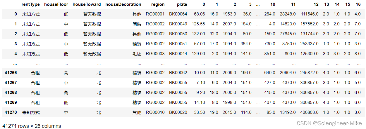
在这里，将这20个特征与6个分类性特征进行合并。

X_new = pd.DataFrame(X_new).reset_index(drop=True)
train_categorical = train[categorical_columns].reset_index(drop=True)
XX = pd.concat([train_categorical,X_new],axis=1)
XX

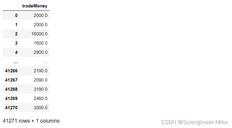
目标值如下：

yy =pd.DataFrame(y).reset_index(drop=True)
yy

在这里，我们准备好我们所需要的训练数据集的特征与标签，测试集的特征，如下：

test_num_features = []
for i in features:
    if test[i].dtype in ["int32","int64","float64"]:
        test_num_features.append(i)
test_num_features = [test_num_features[i] for i in X_new1]
X_TEST1 = test.loc[:,test_num_features]
X_TEST2 = test.loc[:,categorical_columns]
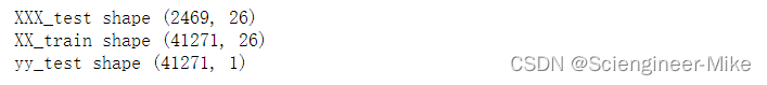
XXX_test = pd.concat([X_TEST2,X_TEST1],axis=1)
print("XXX_test shape",XXX_test.shape)
print("XX_train shape",XX.shape)
print("yy_test shape",yy.shape)

通过lightGBM算法进行建模分析。

# lgb训练模型
from sklearn.model_selection import train_test_split
x_train, x_valid, y_train, y_valid = train_test_split(XX, yy, test_size = 0.25, random_state = 0)
params = {
    
    
    'num_leaves': 31,
    'min_data_in_leaf': 20,
    'min_child_samples':20,
    'objective': 'regression',
    'learning_rate': 0.01,
    "boosting": "gbdt",
    "feature_fraction": 0.8,
    "bagging_freq": 1,
    "bagging_fraction": 0.85,
    "bagging_seed": 23,
    "metric": 'rmse',
    "lambda_l1": 0.2,
    "nthread": 4,
}
lgb_train = lgb.Dataset(x_train, label=y_train, categorical_feature=categorical_columns)
lgb_val = lgb.Dataset(x_valid, label=y_valid, categorical_feature=categorical_columns)
model_LGB = lgb.train(params, lgb_train, 1000)
model_LGB.feature_importance()

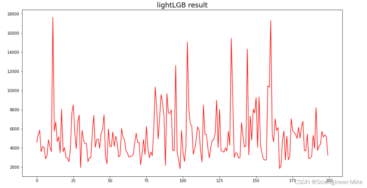
对测试集进行预测。

plt.figure(figsize=(15,8))
plt.plot(model_LGB.predict(XXX_test)[:200],color="red")
plt.title("lightLGB result",size=18)
plt.show()

通过随机森林算法进行建模分析。

因为lightLGB模型可以直接处理分类数据，随机森林则不行。因此，先将数据处理成可以导入随机森林模型的格式。
对分类变量进行编码。

from sklearn.preprocessing import OneHotEncoder

OE = OneHotEncoder(sparse=False, dtype="int32").fit(train[categorical_columns])
train_cate = OE.transform(train[categorical_columns])
test_cate = OE.transform(test[categorical_columns])
train_cate = pd.DataFrame(train_cate)
test_cate = pd.DataFrame(test_cate)
print("编码后的数量shape:",train_cate.shape,test_cate.shape)

将分类特征与数据特征进行堆叠

# 将分类特征和数值型特征进行堆叠
# train
numeric_cate_train = train[num_features].iloc[:,X_new1].reset_index(drop=True)
xxx_train = pd.concat([train_cate,numeric_cate_train],axis=1)
print("堆叠后训练数据集合shape:",xxx_train.shape)
# test
numeric_cate_test = test[num_features].iloc[:,X_new1]
xxx_test = pd.concat([test_cate,numeric_cate_test],axis=1)
print("堆叠后测试数据集合shape:",xxx_test.shape)

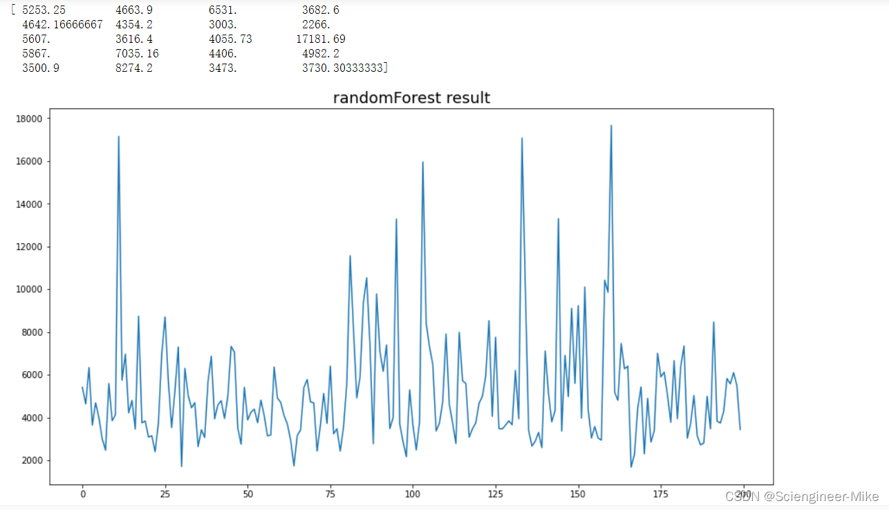
使用随机森林进行训练预测，在训练集上的准确度达到了0.9832。

# 使用随机森林进行训练
model_RFC = RandomForestRegressor().fit(xxx_train,y)
model_RFC.score(xxx_train,y)

# 随机森林预测结果
print(model.predict(xxx_test)[:20])
# 绘制随机森林的预测结果
plt.figure(figsize=(15,8))
plt.plot(model_RFC.predict(xxx_test)[:200])
plt.show()

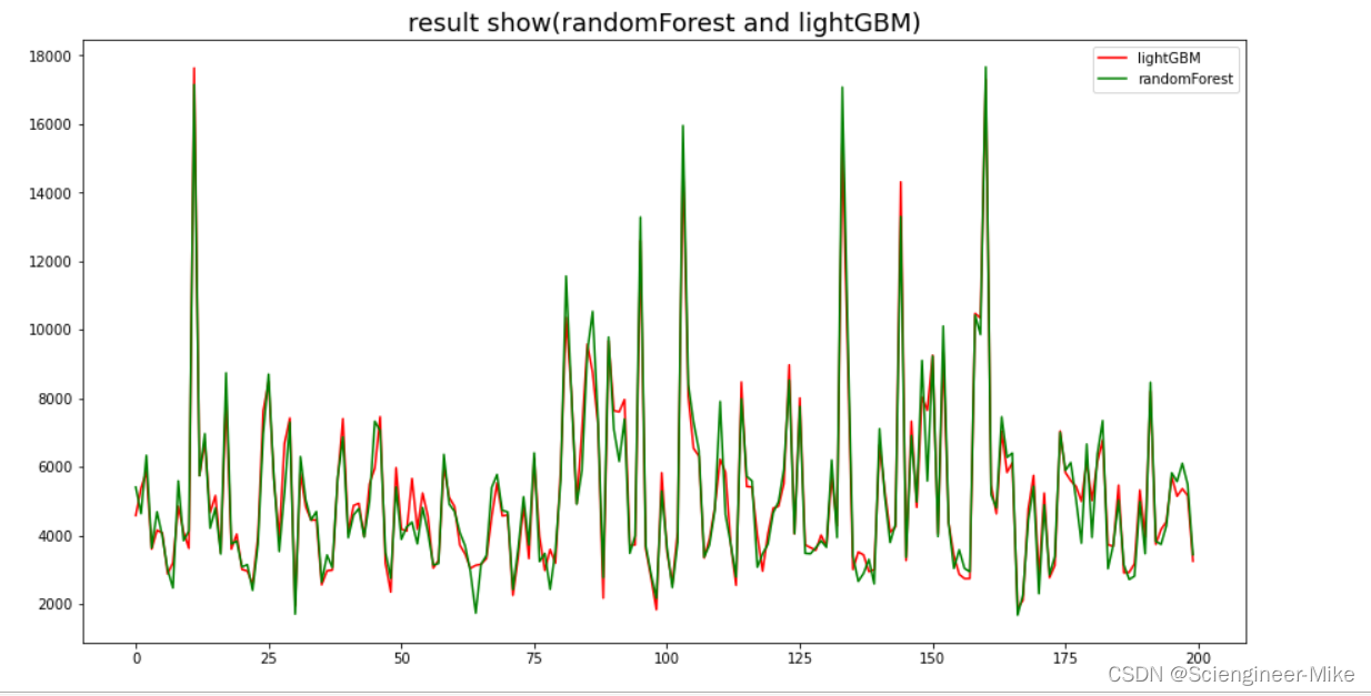
将randomForest和lightGBM两种算法进行结果分析，由结果可以看出，两种算法的结果基本吻合。

plt.figure(figsize=(15,8))
plt.plot(model_LGB.predict(XXX_test)[:200],color="red",label="lightGBM")
plt.plot(model_RFC.predict(xxx_test)[:200],color="green",label="randomForest")
plt.title("result show(randomForest and lightGBM)",size=18)
plt.legend(loc='best')
plt.show()

到此结束，希望对大家有所帮助。