3.4、验证(Validation)
当我们在训练集上指标表现良好时,需要使用验证集来检验一下训练的结果是否存在过拟合现象。
3.4.1、模型与参数的保存
模型的训练可能是一个漫长的过程,在模型训练过程中,以及模型训练完成准备发布时,我们需要保存模型或模型参数,以便在此基础上继续训练,或者把训练好的模型发布上线。
# 保存模型
torch.save(net, './fcn8s.pth')
# 保存模型参数
torch.save(net.state_dict(), './fcn8s.pth')
# 加载整个模型
Net = torch.load('./fcn8s.pth')
# 加载模型参数
net.load_state_dict(torch.load('./fcn8s.pth'))
对于本文,我们仅保存了模型参数,用于继续训练和训练完成后的测试和预测工作。
3.4.2、模型验证
验证是用来评估训练的参数是否过存在拟合现象。验证和测试的过程和代码几乎相同,主要的不同点在于验证阶段不需要进行优化,没有反向传播,梯度下降等优化操作。我们简单的调整训练代码,去掉优化部分,得到如下的验证代码
def validate(self):
    training = self.model.training
    device = torch.device('cuda' if torch.cuda.is_available() else 'cpu')
    criterion = nn.CrossEntropyLoss()
    val_loss = 0.0
    val_acc = 0.0
    mean_iu = 0.0

    self.model.to(device)
    self.model.eval()
    for batch_index, data in enumerate(self.val_loader):
        iteration = batch_index + 1
        std_input = data[0].float() / 255
        if self.transform:
            std_input = self.transform(std_input)
        input = Variable(std_input.to(device))
        target = data[1].float().to(device)
        with torch.no_grad():
            score = self.model(input)

        # metrics
        loss = criterion(score, target)
        if np.isnan(loss.item()):
            raise ValueError('loss is nan while validating')
        val_loss += loss.item()
        pred = OneHotEncoder.encode_score(score)
        cm = Trainer.confusion_matrix(target, pred)
        acc = torch.diag(cm).sum().item() / torch.sum(cm).item()
        val_acc += acc
        iu = torch.diag(cm) / (cm.sum(dim=1) + cm.sum(dim=0) - torch.diag(cm))
        mean_iu += torch.nanmean(iu).item()

    data_len = len(self.val_loader)
    val_loss /= data_len
    val_acc /= data_len
    mean_iu /= data_len

    print(f'validate loss: {val_loss:.5f}, accuracy:{val_acc:.5f}, mean IU:{mean_iu:.5f}')

    if training:
        self.model.train()
上面代码中的model.eval()用来通知pytorch模型,当前处于评估阶段,此时模型中的BatchNormalization, Dropout等算法的行为会发生改变。torch.no_grad()区域内的模型计算不会计算梯度值。在验证代码完成后,我们把模型在训练还是评估阶段的标识还原,这样方便我们接下来进行的混合训练和验证。
3.4.3、混合训练与验证
在指标中,我们列出了一些模型输出结果的度量方法。如果一个模型训练结果的指标符合要求,并且在验证集上同样表现良好,那么我们可以保存模型或模型的参数,之后可直接使用保存下来的模型或参数去做测试和预测工作。
那么我们在是何种情况下,保存模型或模型的参数?这通常依赖于我们要做的具体事情。在语义分割任务中,我们通常选择IOU指标,作为评估保存模型或模型参数的指标。
为了让程序智能为我们选择理想的结果并保存,首先,我们要确保模型的参数,在训练集上训练的结果指标满足需求,然后我们使用此参数进行模型验证,输出验证结果的指标,并保存模型参数。在下一次训练的结果指标满足需求时,如果再次验证的结果指标优于上次保存的指标,那么保存最新的模型参数。最终训练和验证完成后,我们保存的模型的参数,在训练集上的表现符合预期,并且在验证集上的泛化能力最优化。
在trainer的构造函数中定义准确率阈值和中间比对的IOU值
class Trainer(object):
    def __init__(self, model: torch.nn.Module, transform, train_loader: DataLoader, val_loader: DataLoader, class_names, class_colors):
        self.model = model
        self.transform = transform
        self.visualizer = Visualizer(class_names, class_colors)
        self.acc_threshold = 0.95
        self.best_mean_iu = 0
        self.train_loader = train_loader
        self.val_loader = val_loader
在训练代码中,加入混合验证的代码:
if verbose and iteration % iterations_per_epoch == 0:
    mean_acc = train_acc/iterations_per_epoch
    mean_iu = train_iu/iterations_per_epoch
    print(f'epoch {epoch + 1} / {epochs}: loss: {train_loss/iterations_per_epoch:.5f}, accuracy:{mean_acc:.5f}, mean IU:{mean_iu:.5f}')
    if mean_acc > self.acc_threshold:
        self.validate()
最后在模型验证代码中,加入择优保存模型参数的代码
print(f'validate loss: {val_loss:.5f}, accuracy:{val_acc:.5f}, mean IU:{mean_iu:.5f}')
if mean_iu > self.best_mean_iu:
    self.save_model_params()
    self.best_mean_iu = mean_iu
3.5、测试(Test)
当我们训练好了一个模型,我们可以测试模型实际运行的效果. 测试阶段是实际预测的预演,我们通过测试来评估模型正式运行时的效果。通常测试使用的数据,是在训练和验证都没有使用过的数据,这样可以保证测试的结果尽可能接近真实的结果。在测试阶段,我们增加了两个指标:ROC和PR
3.5.1、ROC
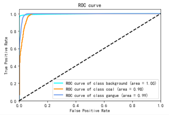
ROC(Receiver Operating Characteristic)指标,可以直观地评价分类器的优劣。ROC指标是多个指标的组合,横坐标FPR(False Positive Rate)也称为误报率。是所有实际为假的样本中被错误地预测为阳性的比例。计算公式为:
FPR = FP / (FP + TN)
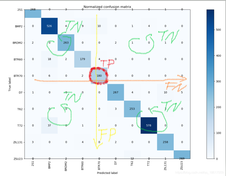
FP在混淆矩阵中是分类所在列中除去斜对角线元素之外所有数值的和, TN在混淆矩阵中是除去分类所在的行和列之外所有的数值之和。
纵坐标TPR(True Positive Rate)也称为召回率,查全率。是所有实际为真的样本中,被正确地预测为阳性的比例。计算公式为:
TPR = TP / ( TP + FN)
TP 在混淆矩阵中是分类所在的斜对角线元素,FN在混淆矩阵中是分类所在行中除去斜对角线元素之外的所有数值之和。
基于预测结果的打分或概率,选定若干个阈值,在不同阈值下的混淆矩阵,对应的TPR和FPR,即构成了一幅ROC曲线图。
ROC曲线图的左下到右上的对角线是随机猜测线,ROC曲线的区域越大,说明预测准确率和越高,如果ROC曲线在对角线下方,说明模型预测的准确率低于随机猜测。
为了绘制各种图表和可视化结果,我们构建了一个可视化的类,使用标签数据和预测结果作为参数来绘制ROC曲线。
这里注意如果是多分类,那么y_pred只能使用概率,否则由于计算某一分类时,并不会参考其它分类的打分,会导致ROC曲线与实际不符。
class Visualizer:
    def __init__(self, class_names, class_colors):
        plt.rcParams['font.sans-serif'] = ['SimHei']
        self.class_names = class_names
        self.n_classes = len(class_names)
        self.class_colors = class_colors

    def draw_roc_auc(self, y_true: Tensor, y_pred: Tensor, title, x_label="False Positive Rate", y_label="True Positive Rate"):
        fpr = dict()
        tpr = dict()
        roc_auc = dict()
        for i in range(self.n_classes):
            fpr[i], tpr[i], _ = roc_curve(y_true[:, i, :, :].view(-1).numpy(), y_pred[:, i, :, :].view(-1).numpy())
            roc_auc[i] = auc(fpr[i], tpr[i])

        for i, color in zip(range(self.n_classes), self.class_colors):
            plt.plot(
                fpr[i],
                tpr[i],
                color=color,
                lw=2,
                label="ROC curve of class {0} (area = {1:0.2f})".format(self.class_names[i], roc_auc[i]),
            )

        plt.plot([0, 1], [0, 1], "k--", lw=2)
        plt.xlim([0.0, 1.0])
        plt.ylim([0.0, 1.05])
        plt.xlabel(x_label)
        plt.ylabel(y_label)
        plt.title(title)
        plt.legend(loc="lower right")
        plt.show()
3.5.2、PR
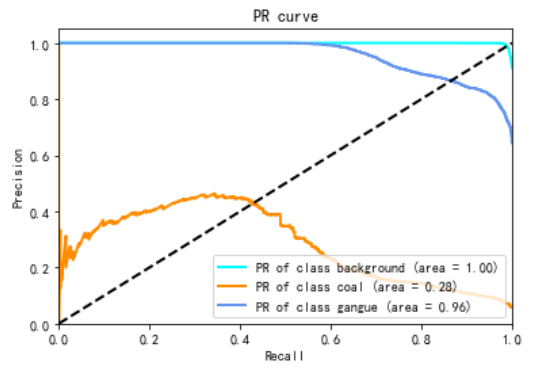
PR(Precision Recall)指标,是精确率(Precision)和召回率(Recall)两个指标的组合。其中横坐标是召回率(Recall),和ROC中的TPR的概念是一致的,表示真的样本中,预测为阳性所在的比例。纵坐标是精确率(Precision),也称为查准率。是所有预测为阳性的样本中,实际为真的比例。计算公式为:
Precision = TP /(TP + FP)
基于预测结果的打分或概率,选定若干个阈值,在不同阈值下的混淆矩阵,对应的Precision和Recall,即构成了一幅PR曲线图。
def draw_pr(self, y_true: Tensor, y_pred: Tensor, title, x_label="Recall", y_label="Precision"):
    precision = dict()
    recall = dict()
    aps = dict()
    for i in range(self.n_classes):
        precision[i], recall[i], thresholds = precision_recall_curve(y_true[:, i, :, :].view(-1).numpy(), y_pred[:, i, :, :].view(-1).numpy())
        aps[i] = average_precision_score(y_true[:, i, :, :].view(-1).numpy(), y_pred[:, i, :, :].view(-1).numpy())

    for i, color in zip(range(self.n_classes), self.class_colors):
        plt.plot(
            recall[i],
            precision[i],
            color=color,
            lw=2,
            label="PR of class {0} (area = {1:0.2f})".format(self.class_names[i], aps[i]),
        )

    plt.plot([0, 1], [0, 1], "k--", lw=2)
    plt.xlim([0.0, 1.0])
    plt.ylim([0.0, 1.05])
    plt.xlabel(x_label)
    plt.ylabel(y_label)
    plt.title(title)
    plt.legend(loc="lower right")
    plt.show()
3.5.3、绘制测试结果
我们可以把测试结果绘制成类似于语义分割标签图片的图像,并对比原标签图像,直观观察分割的结果和实际标签的匹配程度。为了绘制测试结果,我们首先为one-hot编码添加解码能力,把one-hot编码解码成使用不同颜色表示不同分类的图像。
@staticmethod
def decode(input: Tensor, colors: Tensor):
    height, width = input.shape[1:]
    mask = torch.zeros([3, height, width], dtype=torch.long)
    for label_num in range(0, len(colors)):
        index = (input[label_num] == 1)
        mask[:, index] = colors[label_num][:, None]
    return mask
之后使用新增的方法实现绘制测试结果的功能。在一行中分别绘制原图,标签图和预测图。
def draw_result(self, img: Tensor, mask: Tensor, y_pred: Tensor):
    mask_img = OneHotEncoder.decode(mask, self.class_colors)
    pred_img = OneHotEncoder.decode(y_pred, self.class_colors)
    plt.figure(figsize=(12, 5))
    plt.subplot(131)
    plt.imshow(img.permute(1, 2, 0))
    plt.subplot(132)
    plt.imshow(mask_img.permute(1, 2, 0))
    plt.subplot(133)
    plt.imshow(pred_img.permute(1, 2, 0))
    plt.show()
3.5.4、网格化标注
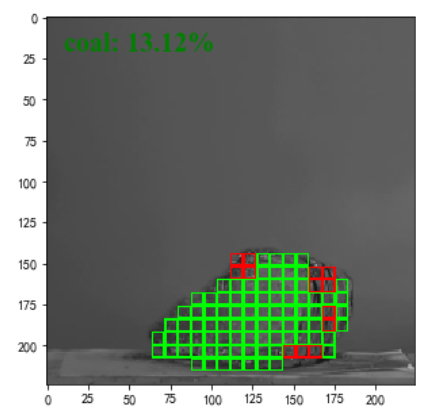
有了预测结果,我们可以根据预测结果在原图或者标签图的基础上做各种叠加处理,用以反馈预测结果在原图上的效果。这里我们尝试使用小网格的方式,在原图之上标注分类的网格区域。
def draw_overlay_grid(self, img: Tensor, overlay_classes, y_pred: Tensor, label):
    font = {'color': 'green',
            'size': 20,
            'family': 'Times New Roman'}
    grid = torch.tensor([
        [0, 0, 0, 0, 0, 0, 0, 0],
        [0, 1, 1, 1, 1, 1, 1, 0],
        [0, 1, 1, 1, 1, 1, 1, 0],
        [0, 1, 1, 1, 1, 1, 1, 0],
        [0, 1, 1, 1, 1, 1, 1, 0],
        [0, 1, 1, 1, 1, 1, 1, 0],
        [0, 1, 1, 1, 1, 1, 1, 0],
        [0, 0, 0, 0, 0, 0, 0, 0]
    ])
    w, h = img.shape[1:]
    k_size = grid.shape[0]
    left, top = 0, 0
    while top < h:
        left = 0
        bottom = min(top + k_size, h)
        while left < w:
            right = min(left + k_size, w)
            sum_pred = torch.sum(y_pred[:, top:bottom, left:right].flatten(1, 2), dim=1)
            klass = sum_pred.argmax()
            if klass in overlay_classes:
                img[:, top:bottom, left:right] = torch.mul(
                    img[:, top:bottom, left:right], grid[0:bottom-top,0:right-left]) + torch.mul(self.class_colors[klass][:,None, None], grid ^ 1)

    plt.figure(figsize=(12, 5))
    plt.imshow(img.permute(1, 2, 0))
    if label:
        plt.text(10, 20, label, fontdict=font)
    plt.show()
4、总结
在本文中,我们介绍了语义分割技术,一些机器学习的技术和概念在语义分割技术中的应用。最后,我们介绍了几种评估指标以及绘制指标图,通过指标图和参数的配合,深入理解语义分割模型,学习准则和优化过程中,各个超参数的意义和影响。整个实验涉及到了许多的Scalar,Vector,Matrix,Tensor之间的运算,需要我们熟练使用pyorch,numpy等框架和库对这些类型的数据进行处理。