从零开始手把手搭建Vision Transformers(Pytorch版本)

更多内容关注公众号“所向披靡的张大刀”

导言

Vision Transformers (ViT)在2020年Dosovitskiy et. al.提出后，在计算机视觉领域逐渐占领主导位置，在图像分类以及目标检测、语义分割等下游任务中获得了很好的性能，掀起transformer系列在CV领域的浪潮。这里将介绍如何从头开始基于Pytorch 框架一步步实现ViT模型。

前言

如果你还没有熟悉自然语言处理（NLP）中使用的Transformer模型，可能会对transformer在CV领域的应用有点懵圈，对ViT模型在图像上的使用不明所以，别担心，这里将实战如何从头开始实现我的第一个 ViT（使用 PyTorch）,开始吧！

定义任务

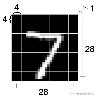
对于小白新手，我们选择入门数据集，我们的MNIST 手写数据集进行图像分类，虽然目标简单，但是我们可以基于该图像分类任务理清ViT模型的整个脉络。简单介绍下MNIST数据集，为是手写数字 ([0–9]) 的数据集，图像均为28x28大小的灰度图。
首先对需要使用的pytorch一些模块导入：

import numpy as np
import torch
import torch.nn as nn
from torch.nn import CrossEntropyLoss
from torch.optim import Adam
from torch.utils.data import DataLoader
from torchvision.datasets.mnist import MNIST
from torchvision.transforms import ToTensor

下面我们来创建main函数，用于预处理MNIST数据集，实例化模型，定义loss，使用Adam优化器，训练50 epochs，然后，在测试集上计算准确率。

def main():
    # Loading data
    transform = ToTensor()

    train_set = MNIST(root='./../datasets', train=True, download=True, transform=transform)
    test_set = MNIST(root='./../datasets', train=False, download=True, transform=transform)

    train_loader = DataLoader(train_set, shuffle=True, batch_size=16)
    test_loader = DataLoader(test_set, shuffle=False, batch_size=16)

    # Defining model and training options
    model = MyViT((1, 28, 28), n_patches=7, hidden_d=20, n_heads=2, out_d=10) # TODO define ViT model 
    N_EPOCHS = 50
    LR = 0.01

    # Training loop
    optimizer = Adam(model.parameters(), lr=LR)
    criterion = CrossEntropyLoss()
    for epoch in range(N_EPOCHS):
        train_loss = 0.0
        for batch in train_loader:
            x, y = batch
            y_hat = model(x)
            loss = criterion(y_hat, y) / len(x)

            train_loss += loss.item()

            optimizer.zero_grad()
            loss.backward()
            optimizer.step()

        print(f"Epoch {
      
      epoch + 1}/{
      
      N_EPOCHS} loss: {
      
      train_loss:.2f}")

 # Test loop
    correct, total = 0, 0
    test_loss = 0.0
    for batch in test_loader:
        x, y = batch
        y_hat = model(x)
        loss = criterion(y_hat, y) / len(x)
        test_loss += loss

        correct += torch.sum(torch.argmax(y_hat, dim=1) == y).item()
        total += len(x)
    print(f"Test loss: {
      
      test_loss:.2f}")
    print(f"Test accuracy: {
      
      correct / total * 100:.2f}%")

搭建好整个训练测试框架后，我们现在来攻克ViT模型的搭建，模型的任务是对（Nx1x28x28）的图像进行分类，我们先定义一个空的nn.Module类，再逐步填充它：

class MyViT(nn.Module):
    def __init__(self):
        # Super constructor
        super(MyViT, self).__init__()

    def forward(self, images):
        pass

ViT架构

因pytorch 以及大多数 DL 框架都提供autograd计算，我们只需要关心实现 ViT 模型的前向传递过程，在训练框架中已经定义了模型的优化器，pytorch框架将负责反向传播梯度并训练模型的参数。

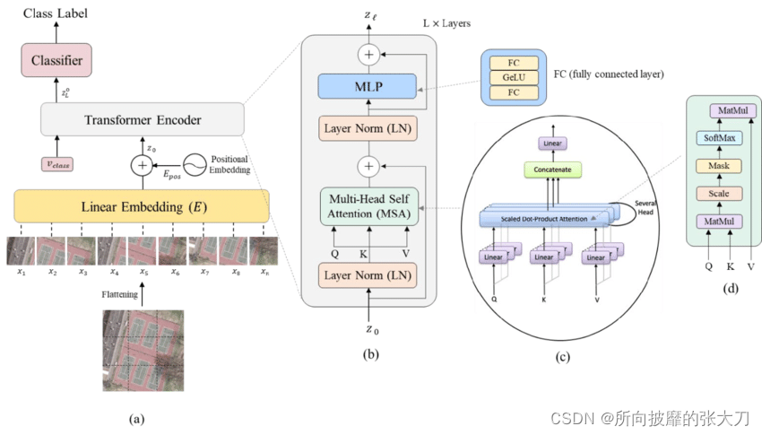
上图展示了ViT的整个模型网络架构，由此我们看到输入图像（a）先被切割成大小相等的patch 子图片，然后每个子图片均被放入到Linear Embedding 中，对每个图片向量做一个全连接操作，做transformer输入的前处理，为啥要加这个Linear Embedding，这里可以参考【1】中作者的解读，这位作者将transformer系列讲的非常详细，墙裂推荐。从Linear Embedding层出来后，加入Positonal encoding 将各个patch在图像中的相对位置信息考虑进去，后面就是transformer Encoder的过程，在之后加入MLP的分类head，输出图像的分类。

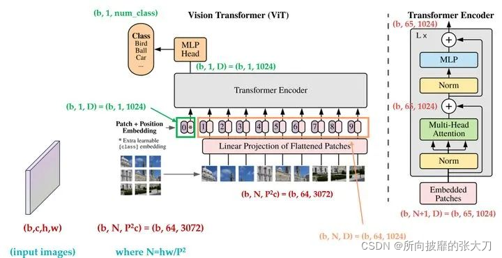
上图是【1】中作者方便大家理解，将前向过程中的各个维度加入。下面我们通过6个主要步骤构建ViT。

Patchifying 和线性映射

Transformer 编码器一开始主要用于NLP这种序列化数据，将它用于CV领域的第一步要处理的是“序列化”图像，这里的处理方式是将一张图像分解成多个子图像，将每个子图像映射成一个向量。
在MNIST数据集上，我们将每个（1x28x28）的图像分成7x7块，每块大小是4x4（如果不能完全整除分块，需要对图像padding填充），这样我们能从单个图像中获得49个子图像。将原图重塑成：
(N, PxP, HxC/P x WxC/P) = (N, 7x7, 4x4) = (N, 49, 16)
请注意，虽然每个子图大小为 1x4x4 ，但我们将其展平为 16 维向量。此外，MNIST只有一个颜色通道。如果有多个颜色通道，它们也会被展平到矢量中。

我们对代码实现上述功能：

class MyViT(nn.Module):
    def __init__(self, input_shape, n_patches=7):
        # Super constructor
        super(MyViT, self).__init__()

        # Input and patches sizes
        self.input_shape = input_shape
        self.n_patches = n_patches
        assert input_shape[1] % n_patches == 0, "Input shape not entirely divisible by number of patches"
        assert input_shape[2] % n_patches == 0, "Input shape not entirely divisible by number of patches"


    def forward(self, images):
        # Dividing images into patches
        n, c, w, h = images.shape
        patches = images.reshape(n, self.n_patches ** 2, self.input_d)
        return patches 

现在我们得到展平后的patches即向量，通过一个线性映射来改变维度，线性映射可以映射到任意向量大小，我们向类构造函数添加一个hidden_d参数，用于“隐藏维度”。这里，使用隐藏维度为8，这样我们将每个 16 维patch映射到一个 8 维patch, 实现代码如下。

class MyViT(nn.Module):
    def __init__(self, input_shape, n_patches=7, hidden_d=8):
        # Super constructor
        super(MyViT, self).__init__()

        # Input and patches sizes
        self.input_shape = input_shape
        self.n_patches = n_patches
        assert input_shape[1] % n_patches == 0, "Input shape not entirely divisible by number of patches"
        assert input_shape[2] % n_patches == 0, "Input shape not entirely divisible by number of patches"
        self.hidden_d = hidden_d

        # 1) Linear mapper
        self.input_d = int(input_shape[0] * self.patch_size[0] * self.patch_size[1])
        self.linear_mapper = nn.Linear(self.input_d, self.hidden_d)

    def forward(self, images):
        # Dividing images into patches
        n, c, w, h = images.shape
        patches = images.reshape(n, self.n_patches ** 2, self.input_d)
         # Running linear layer for tokenization
        tokens = self.linear_mapper(patches)

        return tokens  

添加分类标记

在添加隐藏层后，为了完成分类任务，我们需要添加分类标记，主要原因是参见【1】，这里只做实现。现在可以向我们的模型添加一个参数将我们的 (N, 49, 8)张量转换为 (N, 50, 8) 张量（将特殊标记添加到每个序列）。

class MyViT(nn.Module):
    def __init__(self, input_shape, n_patches=7, hidden_d=8, n_heads=2, out_d=10):
        # Super constructor
        super(MyViT, self).__init__()

        # Input and patches sizes
        self.input_shape = input_shape
        self.n_patches = n_patches
        self.n_heads = n_heads
        assert input_shape[1] % n_patches == 0, "Input shape not entirely divisible by number of patches"
        assert input_shape[2] % n_patches == 0, "Input shape not entirely divisible by number of patches"
        self.hidden_d = hidden_d

        # 1) Linear mapper
        self.input_d = int(input_shape[0] * self.patch_size[0] * self.patch_size[1])
        self.linear_mapper = nn.Linear(self.input_d, self.hidden_d)

        # 2) Classification token
        self.class_token = nn.Parameter(torch.rand(1, self.hidden_d))

    def forward(self, images):
        # Dividing images into patches
        n, c, w, h = images.shape
        patches = images.reshape(n, self.n_patches ** 2, self.input_d)
         # Running linear layer for tokenization
        tokens = self.linear_mapper(patches)
        # Adding classification token to the tokens
        tokens = torch.stack([torch.vstack((self.class_token, tokens[i])) for i in range(len(tokens))])

        return tokens 

请注意，这里 (N,49,8) → (N,50,8) 实现方式可能不是最佳的。另外，请注意分类标记需要放在每个序列的第一个标记位。当我们完成最终 MLP 时，需要对应到对应的位置上。

添加位置编码

位置编码参见transformer模型中位置标明的输入，虽然理论上可以学习这种位置嵌入，但是这块也有人研究过，建议我们可以只添加正弦和余弦波。

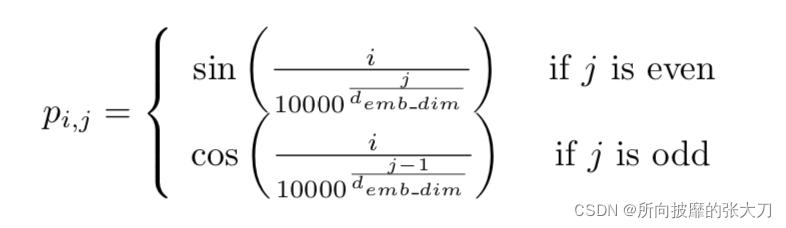
def get_positional_embeddings(sequence_length, d):
    result = torch.ones(sequence_length, d)
    for i in range(sequence_length):
        for j in range(d):
            result[i][j] = np.sin(i / (10000 ** (j / d))) if j % 2 == 0 else np.cos(i / (10000 ** ((j - 1) / d)))
    return resul

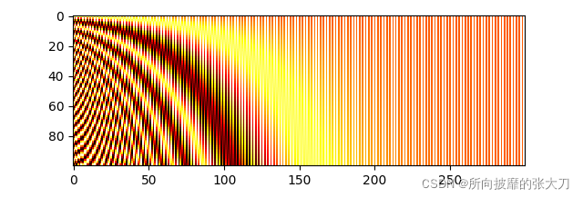
从绘制的热图中，看到所有“水平线”都彼此不同，因此可以区分样本位置。

现在可以在线性映射和添加分类标记后将位置编码添加到模型中：

class MyViT(nn.Module):
    def __init__(self, input_shape, n_patches=7, hidden_d=8, n_heads=2, out_d=10):
        # Super constructor
        super(MyViT, self).__init__()

        # Input and patches sizes
        self.input_shape = input_shape
        self.n_patches = n_patches
        self.n_heads = n_heads
        assert input_shape[1] % n_patches == 0, "Input shape not entirely divisible by number of patches"
        assert input_shape[2] % n_patches == 0, "Input shape not entirely divisible by number of patches"
        self.patch_size = (input_shape[1] / n_patches, input_shape[2] / n_patches)
        self.hidden_d = hidden_d

        # 1) Linear mapper
        self.input_d = int(input_shape[0] * self.patch_size[0] * self.patch_size[1])
        self.linear_mapper = nn.Linear(self.input_d, self.hidden_d)

        # 2) Classification token
        self.class_token = nn.Parameter(torch.rand(1, self.hidden_d))

        # 3) Positional embedding
        # (In forward method)



    def forward(self, images):
        # Dividing images into patches
        n, c, w, h = images.shape
        patches = images.reshape(n, self.n_patches ** 2, self.input_d)

        # Running linear layer for tokenization
        tokens = self.linear_mapper(patches)

        # Adding classification token to the tokens
        tokens = torch.stack([torch.vstack((self.class_token, tokens[i])) for i in range(len(tokens))])

        # Adding positional embedding
        tokens += get_positional_embeddings(self.n_patches ** 2 + 1, self.hidden_d).repeat(n, 1, 1)

        return tokens

由于token的大小为 (N, 50, 8)，我们需要重复 (50, 8) 位置编码矩阵 N 次。

LN, MSA和残差连接

这是最复杂的一步。我们需要先对tokens做层归一化，然后应用多头注意力机制，最后添加一个残差连接（连接LN 之前的输入和多头注意力之后的输出）。

LN

我们通常将LN应用于 (N, d) 输入，其中 d 是维度。直到自己实现 ViT，才发现nn.LayerNorm可以应用于多个维度：

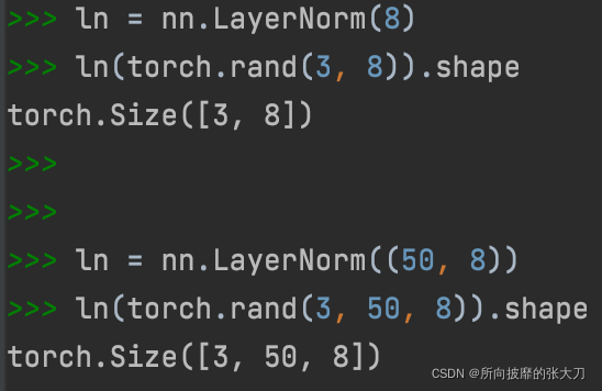
通过 LN 运行 (N, 50, 8) 张量后，每个 50x8 矩阵的均值为 0 和标准差为 1，维度不变。

多头自注意力

我们现在需要实现架构图的子图c。这里就是多头注意力机制，对实现过程不了解的参见【2】，简而言之：对于单个图像，我们希望每个patch都根据与其他patch的某种相似性度量来更新。通过将每个patch（示例中现在是一个 8 维向量）线性映射到 3 个不同的向量：q、k和v（查询、键、值）。然后，对于单个patch，我们将计算其q向量与所有k个向量之间的点积，除以这些向量维度的平方根d，对计算结果softmax激活，最后将计算结果与不同k向量相关联的v向量相乘，整个计算公式如下。

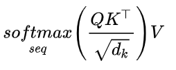
通过这种方式，每个patch获得一个新值，该新值为与其他patch的相似性（在线性映射到q、k和v之后）。整个过程为单头，多头则重复多次整个过程。获得所有结果后，将它们通过线性层连接在一起。

由于执行了相当多的计算，因此为 MSA 创建一个新类：

class MyMSA(nn.Module):
    def __init__(self, d, n_heads=2):
        super(MyMSA, self).__init__()
        self.d = d
        self.n_heads = n_heads

        assert d % n_heads == 0, f"Can't divide dimension {
      
      d} into {
      
      n_heads} heads"

        d_head = int(d / n_heads)
        self.q_mappings = [nn.Linear(d_head, d_head) for _ in range(self.n_heads)]
        self.k_mappings = [nn.Linear(d_head, d_head) for _ in range(self.n_heads)]
        self.v_mappings = [nn.Linear(d_head, d_head) for _ in range(self.n_heads)]
        self.d_head = d_head
        self.softmax = nn.Softmax(dim=-1)

    def forward(self, sequences):
        # Sequences has shape (N, seq_length, token_dim)
        # We go into shape    (N, seq_length, n_heads, token_dim / n_heads)
        # And come back to    (N, seq_length, item_dim)  (through concatenation)
        result = []
        for sequence in sequences:
            seq_result = []
            for head in range(self.n_heads):
                q_mapping = self.q_mappings[head]
                k_mapping = self.k_mappings[head]
                v_mapping = self.v_mappings[head]

                seq = sequence[:, head * self.d_head: (head + 1) * self.d_head]
                q, k, v = q_mapping(seq), k_mapping(seq), v_mapping(seq)

                attention = self.softmax(q @ k.T / (self.d_head ** 0.5))
                seq_result.append(attention @ v)
            result.append(torch.hstack(seq_result))
        return torch.cat([torch.unsqueeze(r, dim=0) for r in result])

请注意，对于每个头部，我们创建了不同的 Q、K 和 V 映射函数（这里为大小为 4x4 的方阵）。

由于输入是大小为 (N, 50, 8) 的序列，我们使用 2 个头，因此我们将在某些时候有 (N, 50, 2, 4) 张量，使用nn.Linear(4, 4 )模块，然后在连接后返回到 (N, 50, 8) 张量。另，使用循环并不是计算多头自注意力的最有效方法，但代码更清晰。

残差连接

将添加一个残差连接，它将我们的原始 (N, 50, 8) 张量添加到在 LN 和 MSA 之后获得的 (N, 50, 8)。

class MyViT(nn.Module):
    def __init__(self, input_shape, n_patches=7, hidden_d=8, n_heads=2, out_d=10):
        # Super constructor
        super(MyViT, self).__init__()

        # Input and patches sizes
        self.input_shape = input_shape
        self.n_patches = n_patches
        self.n_heads = n_heads
        assert input_shape[1] % n_patches == 0, "Input shape not entirely divisible by number of patches"
        assert input_shape[2] % n_patches == 0, "Input shape not entirely divisible by number of patches"
        self.patch_size = (input_shape[1] / n_patches, input_shape[2] / n_patches)
        self.hidden_d = hidden_d

        # 1) Linear mapper
        self.input_d = int(input_shape[0] * self.patch_size[0] * self.patch_size[1])
        self.linear_mapper = nn.Linear(self.input_d, self.hidden_d)

        # 2) Classification token
        self.class_token = nn.Parameter(torch.rand(1, self.hidden_d))

        # 3) Positional embedding
        # (In forward method)

        # 4a) Layer normalization 1
        self.ln1 = nn.LayerNorm((self.n_patches ** 2 + 1, self.hidden_d))

        # 4b) Multi-head Self Attention (MSA) and classification token
        self.msa = MyMSA(self.hidden_d, n_heads)



    def forward(self, images):
        # Dividing images into patches
        n, c, w, h = images.shape
        patches = images.reshape(n, self.n_patches ** 2, self.input_d)

        # Running linear layer for tokenization
        tokens = self.linear_mapper(patches)

        # Adding classification token to the tokens
        tokens = torch.stack([torch.vstack((self.class_token, tokens[i])) for i in range(len(tokens))])

        # Adding positional embedding
        tokens += get_positional_embeddings(self.n_patches ** 2 + 1, self.hidden_d).repeat(n, 1, 1)

        # TRANSFORMER ENCODER BEGINS ###################################
        # NOTICE: MULTIPLE ENCODER BLOCKS CAN BE STACKED TOGETHER ######
        # Running Layer Normalization, MSA and residual connection
        out = tokens + self.msa(self.ln1(tokens))

        return out 

请注意，如果我们现在通过我们的模型运行MNIST的随机 (3, 1, 28, 28) 图像，我们仍然会得到形状为 (3, 50, 8) 的结果。

LN,MLP 和残差连接

继续下面网络，将当前张量再通过另一个 LN 和 MLP 后，通过残差连接，嗯，搭积木这样搭起来。

class MyViT(nn.Module):
    def __init__(self, input_shape, n_patches=7, hidden_d=8, n_heads=2, out_d=10):
        # Super constructor
        super(MyViT, self).__init__()

        # Input and patches sizes
        self.input_shape = input_shape
        self.n_patches = n_patches
        self.n_heads = n_heads
        assert input_shape[1] % n_patches == 0, "Input shape not entirely divisible by number of patches"
        assert input_shape[2] % n_patches == 0, "Input shape not entirely divisible by number of patches"
        self.patch_size = (input_shape[1] / n_patches, input_shape[2] / n_patches)
        self.hidden_d = hidden_d

        # 1) Linear mapper
        self.input_d = int(input_shape[0] * self.patch_size[0] * self.patch_size[1])
        self.linear_mapper = nn.Linear(self.input_d, self.hidden_d)

        # 2) Classification token
        self.class_token = nn.Parameter(torch.rand(1, self.hidden_d))

        # 3) Positional embedding
        # (In forward method)

        # 4a) Layer normalization 1
        self.ln1 = nn.LayerNorm((self.n_patches ** 2 + 1, self.hidden_d))

        # 4b) Multi-head Self Attention (MSA) and classification token
        self.msa = MyMSA(self.hidden_d, n_heads)

        # 5a) Layer normalization 2
        self.ln2 = nn.LayerNorm((self.n_patches ** 2 + 1, self.hidden_d))

        # 5b) Encoder MLP
        self.enc_mlp = nn.Sequential(
            nn.Linear(self.hidden_d, self.hidden_d),
            nn.ReLU()
        )


    def forward(self, images):
        # Dividing images into patches
        n, c, w, h = images.shape
        patches = images.reshape(n, self.n_patches ** 2, self.input_d)

        # Running linear layer for tokenization
        tokens = self.linear_mapper(patches)

        # Adding classification token to the tokens
        tokens = torch.stack([torch.vstack((self.class_token, tokens[i])) for i in range(len(tokens))])

        # Adding positional embedding
        tokens += get_positional_embeddings(self.n_patches ** 2 + 1, self.hidden_d).repeat(n, 1, 1)

        # TRANSFORMER ENCODER BEGINS ###################################
        # NOTICE: MULTIPLE ENCODER BLOCKS CAN BE STACKED TOGETHER ######
        # Running Layer Normalization, MSA and residual connection
        out = tokens + self.msa(self.ln1(tokens))

        # Running Layer Normalization, MLP and residual connection
        out = out + self.enc_mlp(self.ln2(out))
        # TRANSFORMER ENCODER ENDS   ###################################

        return out 

这样，如果我们的模型输入一个随机的 (3, 1, 28, 28)图像张量，out输出仍然会得到一个 (3, 50, 8) 的张量。

分类MLP

最后，我们可以从 N 个序列中只提取分类标记（第一个标记），与添加分类标签的位置对应，并使用每个标记得到 N 个分类。

由于我们决定每个标记是一个 8 维向量，并且由于我们有 10 个可能的数字，我们可以将分类 MLP 实现为一个简单的 8x10 矩阵，并使用 SoftMax 函数激活。

class MyViT(nn.Module):
    def __init__(self, input_shape, n_patches=7, hidden_d=8, n_heads=2, out_d=10):
        # Super constructor
        super(MyViT, self).__init__()

        # Input and patches sizes
        self.input_shape = input_shape
        self.n_patches = n_patches
        self.n_heads = n_heads
        assert input_shape[1] % n_patches == 0, "Input shape not entirely divisible by number of patches"
        assert input_shape[2] % n_patches == 0, "Input shape not entirely divisible by number of patches"
        self.patch_size = (input_shape[1] / n_patches, input_shape[2] / n_patches)
        self.hidden_d = hidden_d

        # 1) Linear mapper
        self.input_d = int(input_shape[0] * self.patch_size[0] * self.patch_size[1])
        self.linear_mapper = nn.Linear(self.input_d, self.hidden_d)

        # 2) Classification token
        self.class_token = nn.Parameter(torch.rand(1, self.hidden_d))

        # 3) Positional embedding
        # (In forward method)

        # 4a) Layer normalization 1
        self.ln1 = nn.LayerNorm((self.n_patches ** 2 + 1, self.hidden_d))

        # 4b) Multi-head Self Attention (MSA) and classification token
        self.msa = MyMSA(self.hidden_d, n_heads)

        # 5a) Layer normalization 2
        self.ln2 = nn.LayerNorm((self.n_patches ** 2 + 1, self.hidden_d))

        # 5b) Encoder MLP
        self.enc_mlp = nn.Sequential(
            nn.Linear(self.hidden_d, self.hidden_d),
            nn.ReLU()
        )

        # 6) Classification MLP
        self.mlp = nn.Sequential(
            nn.Linear(self.hidden_d, out_d),
            nn.Softmax(dim=-1)
        )

    def forward(self, images):
        # Dividing images into patches
        n, c, w, h = images.shape
        patches = images.reshape(n, self.n_patches ** 2, self.input_d)

        # Running linear layer for tokenization
        tokens = self.linear_mapper(patches)

        # Adding classification token to the tokens
        tokens = torch.stack([torch.vstack((self.class_token, tokens[i])) for i in range(len(tokens))])

        # Adding positional embedding
        tokens += get_positional_embeddings(self.n_patches ** 2 + 1, self.hidden_d).repeat(n, 1, 1)

        # TRANSFORMER ENCODER BEGINS ###################################
        # NOTICE: MULTIPLE ENCODER BLOCKS CAN BE STACKED TOGETHER ######
        # Running Layer Normalization, MSA and residual connection
        out = tokens + self.msa(self.ln1(tokens))

        # Running Layer Normalization, MLP and residual connection
        out = out + self.enc_mlp(self.ln2(out))
        # TRANSFORMER ENCODER ENDS   ###################################

        # Getting the classification token only
        out = out[:, 0]

        return self.mlp(out)

我们模型的输出现在是一个 (N, 10) 张量。ok，大功告成！

现在来试试我们的模型表现如何。手动设置 Torch 种子（设置为 0），cpu下运行：

结语

原始 ViT 的作者使用 GeLU 激活函数、多层 MLP，并将多个 Transformer 编码器块堆叠在一起。这里是最简单的乞丐版本，后续大家可以基于此去添加,关注公众号后台回复"vit"获完整代码。

---

论文：https://arxiv.org/abs/2010.11929
参考：
[1] https://zhuanlan.zhihu.com/p/342261872
[2] https://zhuanlan.zhihu.com/p/340149804

更多内容欢迎关注：