https://zhuanlan.zhihu.com/p/38236978
过去的这几年,陆陆续续出现了不少深度学习框架。而在这些框架中,Facebook 发布的 PyTorch 相对较新且很独特的一个,由于灵活、迅速、简单等特点,PyTorch 发展迅猛,受到很多人的青睐。
在 PyTorch 上,我们能够很容易的自定义模型的层级,完全掌控训练过程,包括梯度传播。本文就手把手教你如何用 PyTorch 从零搭建一个完整的图像分类器。
安装 PyTorch
得益于预先内置的库,PyTorch 安装起来相当容易,在所有的系统上都能很好的运行。
在 Windows 系统上安装
只有 CPU:
pip3 install http://download.Pytorch.org/whl/cpu/torch-0.4.0-cp35-cp35m-win_amd64.whl
pip3 install torchvision
有GPU支持
pip3 install http://download.Pytorch.org/whl/cu80/torch-0.4.0-cp35-cp35m-win_amd64.whl
pip3 install torchvision
在Linux系统上安装
只有CPU:
pip3 install torch torchvision
有GPU支持
pip3 install http://download.Pytorch.org/whl/cpu/torch-0.4.0-cp35-cp35m-linux_x86_64.whl
pip3 install torchvision
在OSX系统上安装
只有CPU:
pip3 install torch torchvision
有GPU支持
按照PyTorch官网(https://pytorch.org/)上的详细指令安装。
注意:如果想亲自实践本文的教程,你应该有CUDA GPU。如果没有,也没关系!在https://colab.research.google.com/ 上可以免费使用一个基于云的GPU。
卷积神经网络简介
我们本文要使用的模型为卷积神经网络(CNN),它主要就是由一些卷积层堆叠在一起,通常还会有一些正则层和激活层。卷积神经网络的组成部分总结如下:
- CNN—— 一堆卷积层。
- 卷积层—— 能够检测一定的特征,具有特定数量的通道。
- 通道—— 能够检测图像中的具体特征。
- 核/过滤器—— 每个通道中会被检测到的特征。它有固定的大小,通常为3X3。
简单来说,卷积层相当于一个特征检测层。每个卷积层有特定数目的通道,每个通道能够检测出图像中的具体特征。需要检测的每个特征常常被叫做核(kernel)或过滤器,它们都有固定大小,通常为3X3。
定义模型架构
在PyTorch中,通过能扩展Module类的定制类来定义模型。模型的所有组件可以在torch.nn包中找到。因此,我们只需导入这个包就可以了。这里我们会搭建一个简单的CNN模型,用以分类来自CIFAR 10数据集的RGB图像。该数据集包含了50000张训练图像和10000张测试图像,所有图像大小为32 X 32。
# 导入需要的包
import torch
import torch.nn as nn


class SimpleNet(nn.Module):
    def __init__(self, num_classes=10):
        super(SimpleNet, self).__init__()

        self.conv1 = nn.Conv2d(in_channels=3, out_channels=12, kernel_size=3, stride=1, padding=1)
        self.relu1 = nn.ReLU()

        self.conv2 = nn.Conv2d(in_channels=12, out_channels=12, kernel_size=3, stride=1, padding=1)
        self.relu2 = nn.ReLU()

        self.pool = nn.MaxPool2d(kernel_size=2)

        self.conv3 = nn.Conv2d(in_channels=12, out_channels=24, kernel_size=3, stride=1, padding=1)
        self.relu3 = nn.ReLU()

        self.conv4 = nn.Conv2d(in_channels=24, out_channels=24, kernel_size=3, stride=1, padding=1)
        self.relu4 = nn.ReLU()

        self.fc = nn.Linear(in_features=16 * 16 * 24, out_features=num_classes)

    def forward(self, input):
        output = self.conv1(input)
        output = self.relu1(output)

        output = self.conv2(output)
        output = self.relu2(output)

        output = self.pool(output)

        output = self.conv3(output)
        output = self.relu3(output)

        output = self.conv4(output)
        output = self.relu4(output)

        output = output.view(-1, 16 * 16 * 24)

        output = self.fc(output)

        return output
在上面的代码中,我们首先定义了一个新的类,叫做SimpleNet,它会扩展nn.Module类。在这个类的构造函数中,我们指明了神经网络的全部层。我们的神经网络结构为——ReLU层——卷积层——ReLU层——池化层——卷积层——ReLU层——卷积层——ReLU层——线性层。
我们挨个讲解它们。
卷积层
nn.Conv2d(in_channels=3, out_channels=12, kernel_size=3, stride=1, padding=1)
因为我们的输入为有 3 个通道(红-绿-蓝)的 RGB 图像,我们指明 in_channels 的数量为 3。接着我们想将 12 特征的检测器应用在图像上,所以我们指明 out_channels 的数量为 12。这里我们使用标准大小为 3X3 的核。步幅设定为 1,后面一直是这样,除非你计划缩减图像的维度。将步幅设置为 1,卷积会一次变为 1 像素。最后,我们设定填充(padding)为 1:这样能确保我们的图像以0填充,从而保持输入和输出大小一致。
基本上,你不用太担心目前的步幅和填充大小,重点关注 in_channels 和 out_channels 就好了。
注意这一层的 out_channels 会作为下一层的 in_channels,如下所示:
nn.Conv2d(in_channels=12, out_channels=12, kernel_size=3, stride=1, padding=1)
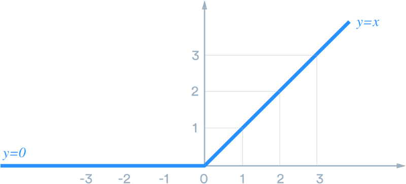
ReLU
这是标准的 ReLU 激活函数,它基本上会将所有输入进来的特征变为 0 或更大的值。简单说,当你用 ReLU 处理输入特征时,任何小于 0 的数字都会被变为 0,其余值保持不变。
MaxPool2d
这一层会通过将 kernel_size 设置为 2、将图像的宽和高减少 2 倍来降低图像的维度。它的基本操作就是在图像的 2X2 区域内取像素最大值,用它来表示整个区域,因此 4 像素就会变成只有 1 个。

线性层
我们的神经网络的最后一层为线性层。这是个标准的全连接层,它会计算每个类的分值——在我们这个例子中是 10 个类。
注意:我们在将最后一个卷积 -ReLU 层中的特征图谱输入图像前,必须把整个图谱压平。最后一层有 24 个输出通道,由于 2X2 的最大池化,在这时我们的图像就变成了16 X 16(32/2 = 16)。我们压平后的图像的维度会是16 x 16 x 24,实现代码如下:
output = output.view(-1, 16 * 16 * 24)
在我们的线性层中,我们必须指明 input_features 的数目同样为 16 x 16 x 24,out_features 的数目应和我们所希望的类的数量一致。
注意在 PyTorch 中定义模型的简单规则。在构造函数中定义层级,在前馈函数中传递所有输入。
希望以上能帮你对如何在 PyTorch 中定义模型有了基本的理解。
模块化
上面的代码虽然酷,但是还不够很酷——如果我们想洗个非常深的神经网络,代码会看着非常臃肿。而让代码保持干净整洁的关键就是模块化。在上面的例子中,我们可以将卷积和 ReLU放在一个单独的模块中,将模块的大部分堆叠在我们的 SimpleNet中。
要做到这点,我们首先以如下方式定义一个新模块:
class Unit(nn.Module):
    def __init__(self, in_channels, out_channels):
        super(Unit, self).__init__()

        self.conv = nn.Conv2d(in_channels=in_channels, kernel_size=3, out_channels=out_channels, stride=1, padding=1)
        self.bn = nn.BatchNorm2d(num_features=out_channels)
        self.relu = nn.ReLU()

    def forward(self, input):
        output = self.conv(input)
        output = self.bn(output)
        output = self.relu(output)

        return output
如上所示,这个单元包含了卷积层-规范层 -ReLU 层。
不想我们所说的第一个例子,这里我们将 BatchNorm2d 放在了 ReLU 前面。规范层会将所有输入标准化为具有零平均值和单位变异数。它会大幅提高 CNN 模型的准确率。
定义好上面的单元后,我们现在将它们堆叠在一起。
class Unit(nn.Module):
    def __init__(self,in_channels,out_channels):
        super(Unit,self).__init__()


        self.conv = nn.Conv2d(in_channels=in_channels,kernel_size=3,out_channels=out_channels,stride=1,padding=1)
        self.bn = nn.BatchNorm2d(num_features=out_channels)
        self.relu = nn.ReLU()

    def forward(self,input):
        output = self.conv(input)
        output = self.bn(output)
        output = self.relu(output)

        return output

class SimpleNet(nn.Module):
    def __init__(self,num_classes=10):
        super(SimpleNet,self).__init__()

        #Create 14 layers of the unit with max pooling in between
        self.unit1 = Unit(in_channels=3,out_channels=32)
        self.unit2 = Unit(in_channels=32, out_channels=32)
        self.unit3 = Unit(in_channels=32, out_channels=32)

        self.pool1 = nn.MaxPool2d(kernel_size=2)

        self.unit4 = Unit(in_channels=32, out_channels=64)
        self.unit5 = Unit(in_channels=64, out_channels=64)
        self.unit6 = Unit(in_channels=64, out_channels=64)
        self.unit7 = Unit(in_channels=64, out_channels=64)

        self.pool2 = nn.MaxPool2d(kernel_size=2)

        self.unit8 = Unit(in_channels=64, out_channels=128)
        self.unit9 = Unit(in_channels=128, out_channels=128)
        self.unit10 = Unit(in_channels=128, out_channels=128)
        self.unit11 = Unit(in_channels=128, out_channels=128)

        self.pool3 = nn.MaxPool2d(kernel_size=2)

        self.unit12 = Unit(in_channels=128, out_channels=128)
        self.unit13 = Unit(in_channels=128, out_channels=128)
        self.unit14 = Unit(in_channels=128, out_channels=128)

        self.avgpool = nn.AvgPool2d(kernel_size=4)

        #Add all the units into the Sequential layer in exact order
        self.net = nn.Sequential(self.unit1, self.unit2, self.unit3, self.pool1, self.unit4, self.unit5, self.unit6
                                 ,self.unit7, self.pool2, self.unit8, self.unit9, self.unit10, self.unit11, self.pool3,
                                 self.unit12, self.unit13, self.unit14, self.avgpool)

        self.fc = nn.Linear(in_features=128,out_features=num_classes)

    def forward(self, input):
        output = self.net(input)
        output = output.view(-1,128)
        output = self.fc(output)
        return output
我们的整个神经网络出来了,它有14个卷积层、14个ReLU层、14个规范层、4个池化层和1个线性层组成,总共62个层!
注意我们把除了全连接层以外的所有层放入一个有序类中,让代码更紧凑些。这会进一步简化前馈函数中的代码。
self.net = nn.Sequential(self.unit1, self.unit2, self.unit3, self.pool1, self.unit4, self.unit5, self.unit6, self.unit7, self.pool2, self.unit8, self.unit9, self.unit10, self.unit11, self.pool3,self.unit12, self.unit13, self.unit14, self.avgpool)
此外,最后一个单元后面的AvgPooling层会计算每个通道中的所有函数的平均值。该单元的输出有128个通道,在池化3次后,我们的32 X 32图像变成了4 X 4。我们以核大小为4使用AvgPool2D,将我们的特征图谱调整为1X1X128。
self.avgpool = nn.AvgPool2d(kernel_size=4)

因此,线性层会有1X1X128=128个输入特征。
self.fc = nn.Linear(in_features=128,out_features=num_classes)

我们同样会压平神经网络的输出,让它有128个特征。
output = output.view(-1,128)
加载和增强数据
得益于torchvision包,数据加载在PyTorch中非常容易。比如,我们加载本文所用的CIFAR10 数据集。
首先,我们需要3个额外的导入语句。
from torchvision.datasets import CIFAR10
from torchvision.transforms import transforms
from torch.utils.data import DataLoader
要加载数据集,我们按照如下步骤操作:
定义即将应用在图像上的转换
用torchvision加载数据集
创建DataLoader的实例来保存照片
代码如下所示:
# 定义训练集的转换,随机翻转图像,剪裁图像,应用平均和标准正常化方法
train_transformations = transforms.Compose([
    transforms.RandomHorizontalFlip(),
    transforms.RandomCrop(32,padding=4),
    transforms.ToTensor(),
    transforms.Normalize((0.5,0.5,0.5), (0.5,0.5,0.5))
])

# 加载训练集
train_set =CIFAR10(root="./data",train=True,transform=train_transformations,download=True)

# 为训练集创建加载程序
train_loader = DataLoader(train_set,batch_size=32,shuffle=True,num_workers=4)
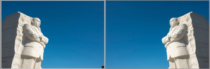
首先,我们用 transform.Compose 输入转换的一个数组。RandomHorizontalFlip 会随机水平翻转照片。RandomCrop 随机剪裁照片。下面是水平剪裁的示例:
最后,两个最重要的步骤:ToTensor 将图像转换为 PyTorch 能够使用的格式;Normalize会让所有像素范围处于-1到+1之间。注意,在声明转换时,ToTensor 和 Normalize 必须和前面定义的顺序一致。主要是因为在输入图像上也应用了其它的转换,比如 PIL 图像处理。
数据增强能帮助模型正确地分类图像,不用考虑图像的展示角度。
接着,我们用 CIFAR10 类加载训练集,最终我们为训练集创建一个加载程序,指定批次大小为32张图像。
在测试集中重复此步骤,只是转换只包括 ToTensor 和 Normalize。我们在测试集中不用其它类型的转换。
# 定义测试集的转换
test_transformations = transforms.Compose([
    transforms.ToTensor(),
    transforms.Normalize((0.5, 0.5, 0.5), (0.5, 0.5, 0.5))

])

# 加载测试集,注意这里的train设为false
test_set = CIFAR10(root="./data", train=False, transform=test_transformations, download=True)

# 为测试集创建加载程序,注意这里的shuffle设为false
test_loader = DataLoader(test_set, batch_size=32, shuffle=False, num_workers=4)
你首次运行此代码时,大约会有 179MB 的数据集加载到你的系统中。
训练模型
用 PyTorch 训练神经网络非常清晰明确,你能区安全控制控制训练过程。我们一步一步解释。
以如下命令导入 Adam 优化器:
from torch.optim import Adam
第一步:初始化模型,创建优化器和损失函数
from torch.optim import Adam


# 检查GPU是否可用
cuda_avail = torch.cuda.is_available()

# 创建模型,优化器和损失函数
model = SimpleNet(num_classes=10)

# 若GPU可用,将模型移往GPU
if cuda_avail:
    model.cuda()

# 定义优化器和损失函数
optimizer = Adam(model.parameters(), lr=0.001, weight_decay=0.0001)
loss_fn = nn.CrossEntropyLoss()
第二步:写一个函数调整学习率
创建一个学习率调整函数,每30个周期将学习率除以10。
# Create a learning rate adjustment function that divides the learning rate by 10 every 30 epochs
def adjust_learning_rate(epoch):
    lr = 0.001

    if epoch > 180:
        lr = lr / 1000000
    elif epoch > 150:
        lr = lr / 100000
    elif epoch > 120:
        lr = lr / 10000
    elif epoch > 90:
        lr = lr / 1000
    elif epoch > 60:
        lr = lr / 100
    elif epoch > 30:
        lr = lr / 10

    for param_group in optimizer.param_groups:
        param_group["lr"] = lr
该函数会在每30个周期后将学习率除以10.
第三步:写出函数保存和评估模型
def save_models(epoch):
    torch.save(model.state_dict(), "cifar10model_{}.model".format(epoch))
print("Chekcpoint saved")

def test():
    model.eval()
    test_acc = 0.0
    for i, (images, labels) in enumerate(test_loader):

        if cuda_avail:
            images = Variable(images.cuda())
            labels = Variable(labels.cuda())

        # Predict classes using images from the test set
        outputs = model(images)
        _, prediction = torch.max(outputs.data, 1)

        test_acc += torch.sum(prediction == labels.data)

    # Compute the average acc and loss over all 10000 test images
    test_acc = test_acc / 10000

return test_acc
为了能评估模型在测试集上准确度,我们迭代测试加载程序。在每一步,我们会把图像和标签移往GPU,在Variable中将它们封装。将图像传入模型中以获取预测值。选择最大预测值,然后和实际类进行比较,以获取准确率。最后,我们返回平均准确率。
第四步:写出训练函数
def train(num_epochs):
    best_acc = 0.0

    for epoch in range(num_epochs):
        model.train()
        train_acc = 0.0
        train_loss = 0.0
        for i, (images, labels) in enumerate(train_loader):
            # 若GPU可用,将图像和标签移往GPU
            if cuda_avail:
                images = Variable(images.cuda())
                labels = Variable(labels.cuda())

            # 清除所有累积梯度
            optimizer.zero_grad()
            # 用来自测试集的图像预测类
            outputs = model(images)
            # 根据实际标签和预测值计算损失
            loss = loss_fn(outputs, labels)
            # 传播损失
            loss.backward()

            # 根据计算的梯度调整参数
            optimizer.step()

            train_loss += loss.cpu().data[0] * images.size(0)
            _, prediction = torch.max(outputs.data, 1)

            train_acc += torch.sum(prediction == labels.data)

        # 调用学习率调整函数
        adjust_learning_rate(epoch)

        # 计算模型在50000张训练图像上的准确率和损失值
        train_acc = train_acc / 50000
        train_loss = train_loss / 50000

        # 用测试集评估
        test_acc = test()

        # 若测试准确率高于当前最高准确率,则保存模型
        if test_acc > best_acc:
            save_models(epoch)
            best_acc = test_acc

        # 打印度量
        print("Epoch {}, Train Accuracy: {} , TrainLoss: {} , Test Accuracy: {}".format(epoch, train_acc, train_loss,
上面的训练函数虽然有注释,但有些地方可能仍然会让你感到很困惑。我们详细解释一下上面到底发生了什么。
首先我们循环训练集的加载程序:
for i, (images,labels) in enumerate(train_loader):

接着,如果可以用GPU,我们就将图像和标签移往GPU:
if cuda_avail:
    images = Variable(images.cuda())
labels = Variable(labels.cuda())
下一行就是清除当前所有的累积梯度:
optimizer.zero_grad()
这很重要,因为根据每个批次累积的梯度神经网络的权重是可以调整的,在每个新的批次内梯度必须重新设置为0,因此之前批次中的图像不会将梯度传播入新的批次。
在接下来的步骤中,我们将图像传入模型中。模型会返回预测值,然后我们将预测值和实际标签输入损失函数中。
我们调用 loss.backward() 来传播梯度,然后根据传播的梯度调用 optimizer.step() 来修正模型的参数。
这些就是训练的主要步骤。
剩余的代码用于计算度量:
train_loss += loss.cpu().data[0] * images.size(0)
_, prediction = torch.max(outputs.data, 1)

train_acc += torch.sum(prediction == labels.data)
这里我们检索实际损失,然后获取最大预测类。最后,我们将所有批次中的正确预测值相加,把所得值添加入整个 train_acc 中。
更重要的是,我们会一直追踪最高的准确率,如果当前测试准确率高于我们的最好成绩,我们就调用保存模型的函数。
GitHub 完整代码地址:
https://gist.github.com/johnolafenwa/96b3322aabb61d4d36fd870a77f02aa3
运行此代码 35 个周期后,你应该会得到超过 90% 的准确率。
用保存的模型进行推断
模型经过训练后,就可以用来对新的图像进行推断。
执行推断过程的步骤如下:
- 定义和初始化你在训练阶段构造的同一模型
- 将保存的检查点加载到模型中
- 从文件系统中选择一张图像
- 让图像通过模型,检索最高预测值
- 将预测的类数目转换为类名
我们用具有预训练的 ImageNet 权重的 Squeeze 模型来解释一下。它几乎能让我们选择任何图形,并获取图像的预测值。
Torchvision 提供预定义模型,涵盖大部分主流架构。
首先,导入所有需要的包和类,创建Squeezenet模型的实例,
# 导入需要的包
import torch
import torch.nn as nn
from torchvision.transforms import transforms
from torch.autograd import Variable
from torchvision.models import squeezenet1_1
import requests
import shutil
from io import open
import os
from PIL import Image
import json


model = squeezenet1_1(pretrained=True)
model.eval()
注意,在上面的代码中,通过将pretrained设为True,Squeezenet模型在你首次运行函数时就会被下载。模型的大小只有4.7 MB。
接着,创建一个预测函数,如下:
def predict_image(image_path):
    print("Prediction in progress")
    image = Image.open(image_path)

    # Define transformations for the image, should (note that imagenet models are trained with image size 224)
    transformation = transforms.Compose([
        transforms.CenterCrop(224),
        transforms.ToTensor(),
        transforms.Normalize((0.5, 0.5, 0.5), (0.5, 0.5, 0.5))

    ])

    # 预处理图像
    image_tensor = transformation(image).float()

    # 额外添加一个批次维度,因为PyTorch将所有的图像当做批次
    image_tensor = image_tensor.unsqueeze_(0)

    if torch.cuda.is_available():
        image_tensor.cuda()

    # 将输入变为变量
    input = Variable(image_tensor)

    # 预测图像的类
    output = model(input)

    index = output.data.numpy().argmax()

return index
上面的代码包含了我们在训练和评估模型阶段所用的同样组件。可以查看上面代码中的注释。
最后,在主函数中进行预测,我们从网上下载一张图像,保存在硬盘上。我们同样下载将所有类索引映射为实际类名的类映射。这是因为我们的模型会根据预测类名的编码方式,返回预测类的索引,然后从索引-类映射中检索实际的类名。
在这之后,我们用保存的图像运行预测函数,用保存的类映射获取正确的类名。
if __name__ == "__main__":

    imagefile = "image.png"

    imagepath = os.path.join(os.getcwd(), imagefile)
    # Donwload image if it doesn't exist
    if not os.path.exists(imagepath):
        data = requests.get(
            "https://github.com/OlafenwaMoses/ImageAI/raw/master/images/3.jpg", stream=True)

        with open(imagepath, "wb") as file:
            shutil.copyfileobj(data.raw, file)

        del data

    index_file = "class_index_map.json"

    indexpath = os.path.join(os.getcwd(), index_file)
    # Donwload class index if it doesn't exist
    if not os.path.exists(indexpath):
        data = requests.get('https://github.com/OlafenwaMoses/ImageAI/raw/master/imagenet_class_index.json')

        with open(indexpath, "w", encoding="utf-8") as file:
            file.write(data.text)

    class_map = json.load(open(indexpath))

    # run prediction function annd obtain prediccted class index
    index = predict_image(imagepath)

    prediction = class_map[str(index)][1]

print("Predicted Class ", prediction)
这是推断过程的完整代码:
# Import needed packages
import torch
import torch.nn as nn
from torchvision.transforms import transforms
import matplotlib.pyplot as plt
import numpy as np
from torch.autograd import Variable
from torchvision.models import squeezenet1_1
import torch.functional as F
import requests
import shutil
from io import open
import os
from PIL import Image
import json

""" Instantiate model, this downloads tje 4.7 mb  squzzene the first time it is called.
To use with your own model, re-define your trained networks ad load weights as below

checkpoint = torch.load("pathtosavemodel")
model = SimpleNet(num_classes=10)


model.load_state_dict(checkpoint)
model.eval()
"""


model = squeezenet1_1(pretrained=True)
model.eval()


def predict_image(image_path):
    print("Prediction in progress")
    image = Image.open(image_path)

    # Define transformations for the image, should (note that imagenet models are trained with image size 224)
    transformation = transforms.Compose([
        transforms.CenterCrop(224),
        transforms.ToTensor(),
        transforms.Normalize((0.5, 0.5, 0.5), (0.5, 0.5, 0.5))

    ])

    # Preprocess the image
    image_tensor = transformation(image).float()

    # Add an extra batch dimension since pytorch treats all images as batches
    image_tensor = image_tensor.unsqueeze_(0)

    if torch.cuda.is_available():
        image_tensor.cuda()

    # Turn the input into a Variable
    input = Variable(image_tensor)

    # Predict the class of the image
    output = model(input)

    index = output.data.numpy().argmax()

    return index


if __name__ == "__main__":

    imagefile = "image.png"

    imagepath = os.path.join(os.getcwd(), imagefile)
    # Donwload image if it doesn't exist
    if not os.path.exists(imagepath):
        data = requests.get(
            "https://github.com/OlafenwaMoses/ImageAI/raw/master/images/3.jpg", stream=True)

        with open(imagepath, "wb") as file:
            shutil.copyfileobj(data.raw, file)

        del data

    index_file = "class_index_map.json"

    indexpath = os.path.join(os.getcwd(), index_file)
    # Donwload class index if it doesn't exist
    if not os.path.exists(indexpath):
        data = requests.get('https://github.com/OlafenwaMoses/ImageAI/raw/master/imagenet_class_index.json')

        with open(indexpath, "w", encoding="utf-8") as file:
            file.write(data.text)

    class_map = json.load(open(indexpath))

    # run prediction function annd obtain prediccted class index
    index = predict_image(imagepath)

    prediction = class_map[str(index)][1]

    print("Predicted Class ", prediction)
上面所用的样本图像就是下面这张:
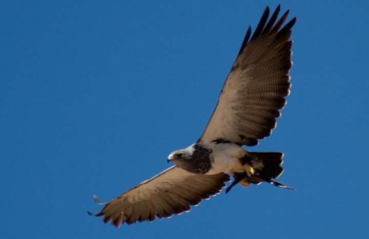
这张照片来自ImageAI。如果你想用自己搭建的网络进行推断,比如我们前面搭建的SimpleNet,你只需替换模型的加载部分:
checkpoint = torch.load("pathtosavemodel")
model = SimpleNet(num_classes=10)


model.load_state_dict(checkpoint)
model.eval()
注意,如果你的模型使用ImageNet训练的,那么你的num_classes必须为1000而不是10.
代码的所有其它部分维持一致,只有一点不同——如果我们以使用CIFAR10训练的模型进行预测,那么在转换中,要将transforms.CenterCrop(224)改变为transforms.Resize(32)。
不过,如果你的模型是用ImageNet训练的,就不用改了。
结语
本文我们介绍了如何用PyTorch搭建一个图像分类器,以及如何用训练后的模型对其它数据做出预测。
关于PyTorch和TensorFlow的不同之处,可以参考我们的这篇文章:
https://zhuanlan.zhihu.com/p/37102973
参考资料:
https://heartbeat.fritz.ai/basics-of-image-classification-with-pytorch-2f8973c51864